Some diagnostics for a fitted qgam model

Takes a fitted gam object produced by qgam() and produces some diagnostic information about the fitting procedure and results. It is partially based on mgcv::gam.check.

# S3 method for qgam
check(obj, nbin = 10, lev = 0.05, ...)

Arguments

obj	the output of a qgam() call.
nbin	number of bins used in the internal call to cqcheck().
lev	the significance levels used by cqcheck(), which determines the width of the confidence intervals.
...	extra arguments to be passed to plot()

Value

Simply produces some plots and prints out some diagnostics.

Details

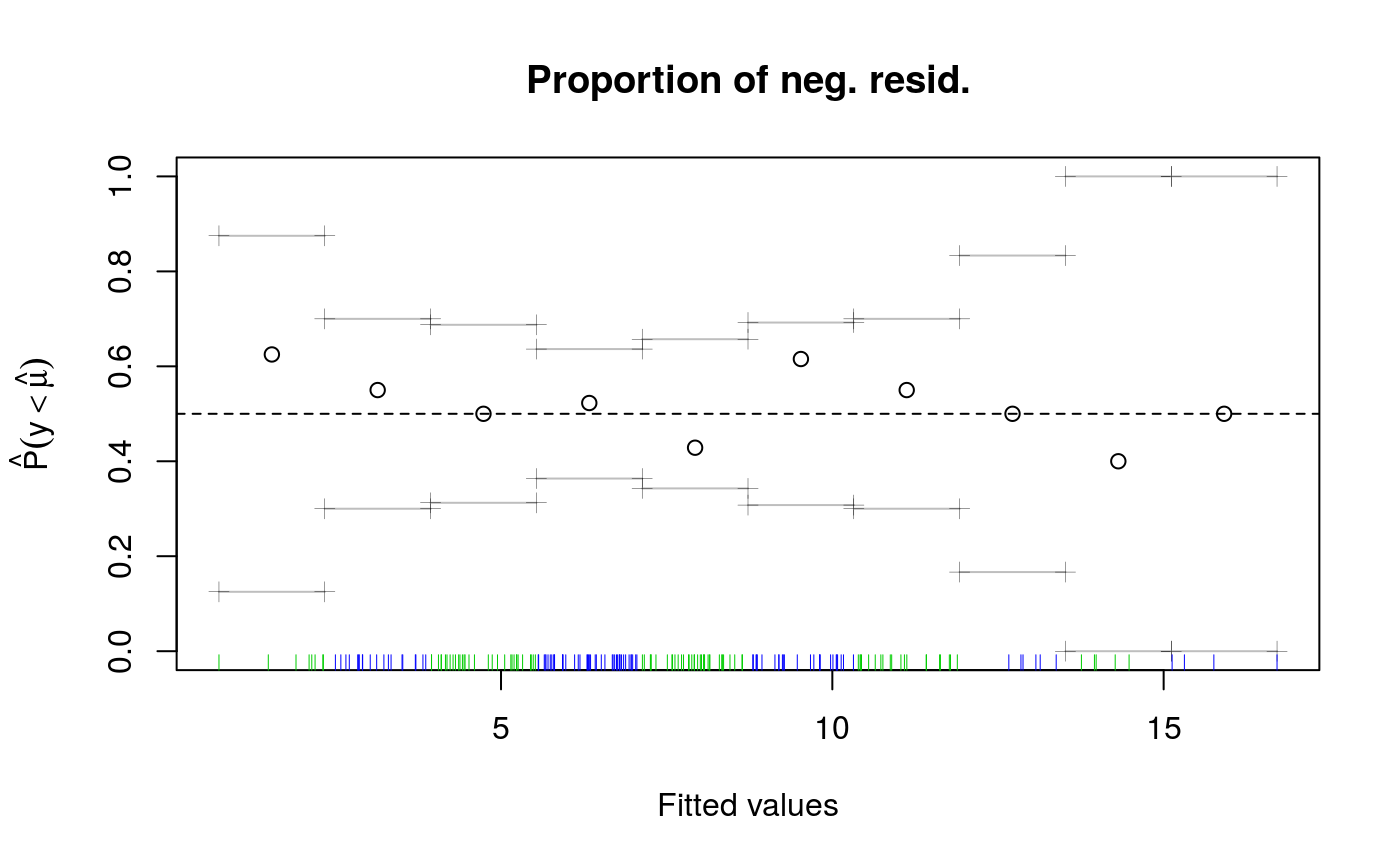
This function provides two plots. The first shows how the number of responses falling below the fitted quantile (y-axis) changes with the fitted quantile (x-axis). To be clear: if the quantile is fixed to, say, 0.5 we expect 50% of the responses to fall below the fit. See ?cqcheck() for details. The second plot related to |F(hat(mu)) - F(mu0)|, which is the absolute bias attributable to the fact that qgam is using a smoothed version of the pinball-loss. The absolute bias is evaluated at each observation, and an histogram is produced. See Fasiolo et al. (2017) for details. The function also prints out the integrated absolute bias, and the proportion of observations lying below the regression line. It also provides some convergence diagnostics (regarding the optimization), which are the same as in mgcv::gam.check. It reports also the maximum (k') and the selected degrees of freedom of each smooth term.

References

Fasiolo, M., Goude, Y., Nedellec, R. and Wood, S. N. (2017). Fast calibrated additive quantile regression. Available at https://arxiv.org/abs/1707.03307.

Examples

library(qgam)
set.seed(0)
dat <- gamSim(1, n=200)
#> Gu & Wahba 4 term additive model
b<-qgam(y~s(x0)+s(x1)+s(x2)+s(x3), data=dat, qu = 0.5)
#> Estimating learning rate. Each dot corresponds to a loss evaluation. 
#> qu = 0.5...............done 
plot(b, pages=1)
check.qgam(b, pch=19, cex=.3)
#> Theor. proportion of neg. resid.: 0.5   Actual proportion: 0.52
#> Integrated absolute bias |F(mu) - F(mu0)| = 0.04500293
#> Method: REML   Optimizer: outer newton
#> full convergence after 6 iterations.
#> Gradient range [-0.0001503744,2.710312e-05]
#> (score 454.5555 & scale 1).
#> Hessian positive definite, eigenvalue range [0.02110521,2.627179].
#> Model rank =  37 / 37 
#> 
#> Basis dimension (k) check: if edf is close too k' (maximum possible edf) 
#> it might be worth increasing k. 
#> 
#>       k'  edf
#> s(x0)  9 2.75
#> s(x1)  9 2.58
#> s(x2)  9 7.44
#> s(x3)  9 1.21