This R package offers methods for fitting additive quantile regression models based on splines, using the methods described in Fasiolo et al., 2017.

The main fitting functions are:

qgam() fits an additive quantile regression model to a single quantile. Very similar to mgcv::gam(). It returns an object of class qgam, which inherits from mgcv::gamObject.
mqgam() fits the same additive quantile regression model to several quantiles. It is more efficient that calling qgam() several times, especially in terms of memory usage.
tuneLearn() useful for tuning the learning rate of the Gibbs posterior. It evaluates a calibration loss function on a grid of values provided by the user.
tuneLearnFast() similar to tuneLearn(), but here the learning rate is selected by minimizing the calibration loss, using Brent method.

A first example: smoothing the motorcycle dataset

Let’s start with a simple example. Here we are fitting a regression model with an adaptive spline basis to quantile 0.8 of the motorcycle dataset.

library(qgam); library(MASS)
if( suppressWarnings(require(RhpcBLASctl)) ){ blas_set_num_threads(1) } # Optional

fit <- qgam(accel~s(times, k=20, bs="ad"), 
            data = mcycle, 
            qu = 0.8)

## Estimating learning rate. Each dot corresponds to a loss evaluation. 
## qu = 0.8............done

# Plot the fit
xSeq <- data.frame(cbind("accel" = rep(0, 1e3), "times" = seq(2, 58, length.out = 1e3)))
pred <- predict(fit, newdata = xSeq, se=TRUE)
plot(mcycle$times, mcycle$accel, xlab = "Times", ylab = "Acceleration", ylim = c(-150, 80))
lines(xSeq$times, pred$fit, lwd = 1)
lines(xSeq$times, pred$fit + 2*pred$se.fit, lwd = 1, col = 2)
lines(xSeq$times, pred$fit - 2*pred$se.fit, lwd = 1, col = 2)

qgam automatically calls tuneLearnFast to select the learning rate. The results of the calibrations are stored in fit$calibr. We can check whether the optimization succeded as follows:

check(fit$calibr, 2)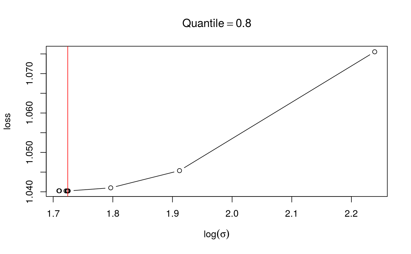

The plot suggest that the calibration criterion has a single minimum, and that the optimizer has converged to its neighbourhood. Alternatively, we could have selected the learning rate by evaluating the loss function on a grid.

set.seed(6436)
cal <- tuneLearn(accel~s(times, k=20, bs="ad"), 
                 data = mcycle, 
                 qu = 0.8,
                 lsig = seq(1, 3, length.out = 20), 
                 control = list("progress" = "none")) #<- sequence of values for learning rate
                 
check(cal)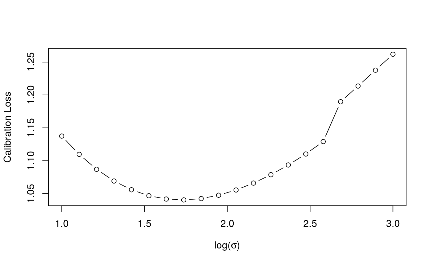

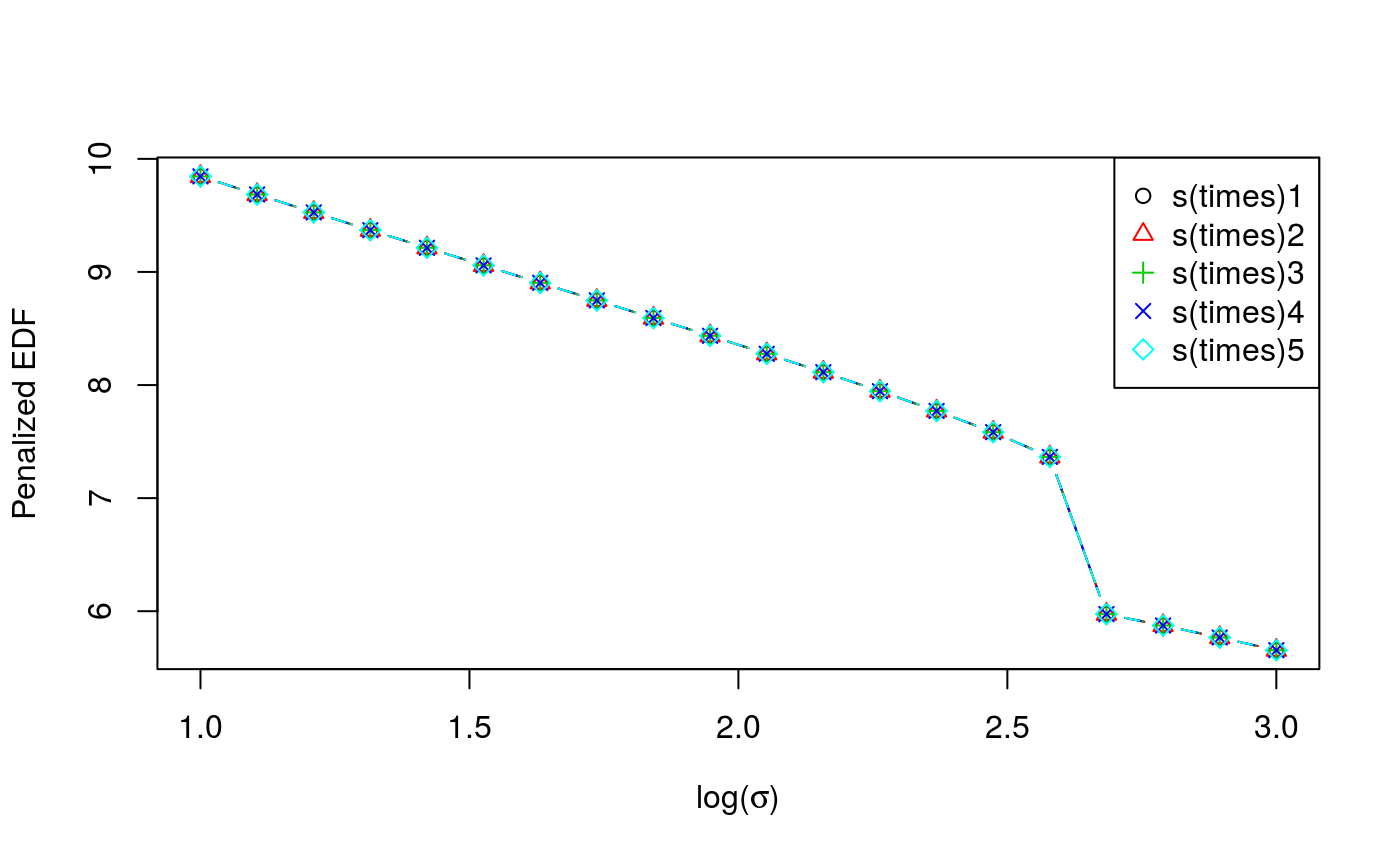Here the generic check function produces a different output. The first plot is the calibration criterion as a function of $log(\sigma)$, which should look fairly smooth. The second plot shows how the effective degrees of freedom (EDF) vary with $log(\sigma)$. Notice that here we are using an adaptive smoother, which includes five smoothing parameters.

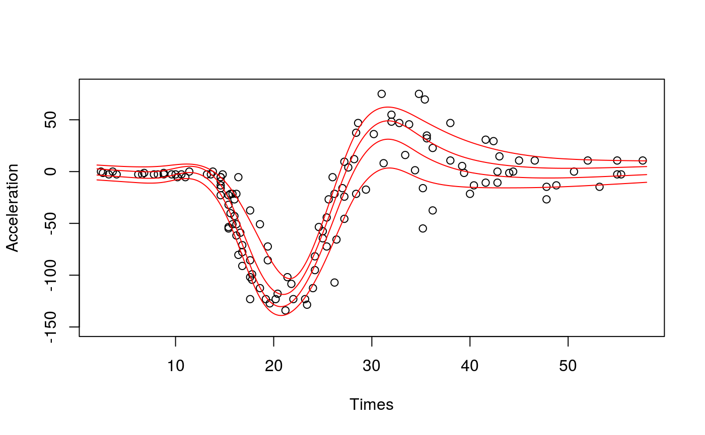
We might want to fit several quantiles at once. This can be done with mqgam.

quSeq <- c(0.2, 0.4, 0.6, 0.8)
set.seed(6436)
fit <- mqgam(accel~s(times, k=20, bs="ad"), 
             data = mcycle, 
             qu = quSeq)

## Estimating learning rate. Each dot corresponds to a loss evaluation. 
## qu = 0.4..........done 
## qu = 0.6...........done 
## qu = 0.2............done 
## qu = 0.8..........done

To save memory mqgam does not return one mgcv::gamObject for each quantile, but it avoids storing some redundant data (such as several copies of the design matrix). The output of mqgam can be manipulated using the qdo function.

# Plot the data
xSeq <- data.frame(cbind("accel" = rep(0, 1e3), "times" = seq(2, 58, length.out = 1e3)))
plot(mcycle$times, mcycle$accel, xlab = "Times", ylab = "Acceleration", ylim = c(-150, 80))

# Predict each quantile curve and plot
for(iq in quSeq){
  pred <- qdo(fit, iq, predict, newdata = xSeq)
  lines(xSeq$times, pred, col = 2)
}

Using qdo we can print out the summary for each quantile, for instance:

# Summary for quantile 0.4
qdo(fit, qu = 0.4, summary)

## 
## Family: elf 
## Link function: identity 
## 
## Formula:
## accel ~ s(times, k = 20, bs = "ad")
## 
## Parametric coefficients:
##             Estimate Std. Error z value Pr(>|z|)    
## (Intercept)  -31.181      1.832  -17.02   <2e-16 ***
## ---
## Signif. codes:  0 '***' 0.001 '**' 0.01 '*' 0.05 '.' 0.1 ' ' 1
## 
## Approximate significance of smooth terms:
##            edf Ref.df Chi.sq p-value    
## s(times) 8.968  10.35  666.4  <2e-16 ***
## ---
## Signif. codes:  0 '***' 0.001 '**' 0.01 '*' 0.05 '.' 0.1 ' ' 1
## 
## R-sq.(adj) =  0.781   Deviance explained = 69.9%
## -REML = 609.58  Scale est. = 1         n = 133

Notice that here the generic function summary is calling summary.gam, because summary.qgam has not been implemented yet. Hence one cannot quite rely on the p-value provided by this function, because their are calculated using result that apply to parametric, not quantile, regression.

Dealing with heteroscedasticity

Let us simulate some data from an heteroscedastic model.

set.seed(651)
n <- 2000
x <- seq(-4, 3, length.out = n)
X <- cbind(1, x, x^2)
beta <- c(0, 1, 1)
sigma =  1.2 + sin(2*x)
f <- drop(X %*% beta)
dat <- f + rnorm(n, 0, sigma)
dataf <- data.frame(cbind(dat, x))
names(dataf) <- c("y", "x")
   
qus <- seq(0.05, 0.95, length.out = 5)
plot(x, dat, col = "grey", ylab = "y")
for(iq in qus){ lines(x, qnorm(iq, f, sigma)) }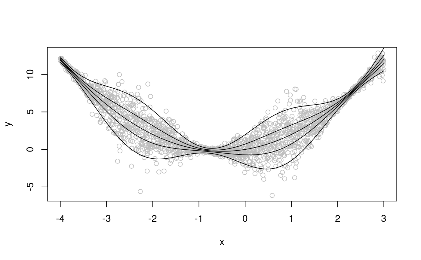

We now fit ten quantiles between 0.05 and 0.95, using a quantile GAM with scalar learning rate.

fit <- mqgam(y~s(x, k = 30, bs = "cr"), 
             data = dataf,
             qu = qus)

## Estimating learning rate. Each dot corresponds to a loss evaluation. 
## qu = 0.5........done 
## qu = 0.725.......done 
## qu = 0.275.........done 
## qu = 0.95................done 
## qu = 0.05...............done

qus <- seq(0.05, 0.95, length.out = 5)
plot(x, dat, col = "grey", ylab = "y")
for(iq in qus){ 
 lines(x, qnorm(iq, f, sigma), col = 2)
 lines(x, qdo(fit, iq, predict))
}
legend("top", c("truth", "fitted"), col = 2:1, lty = rep(1, 2))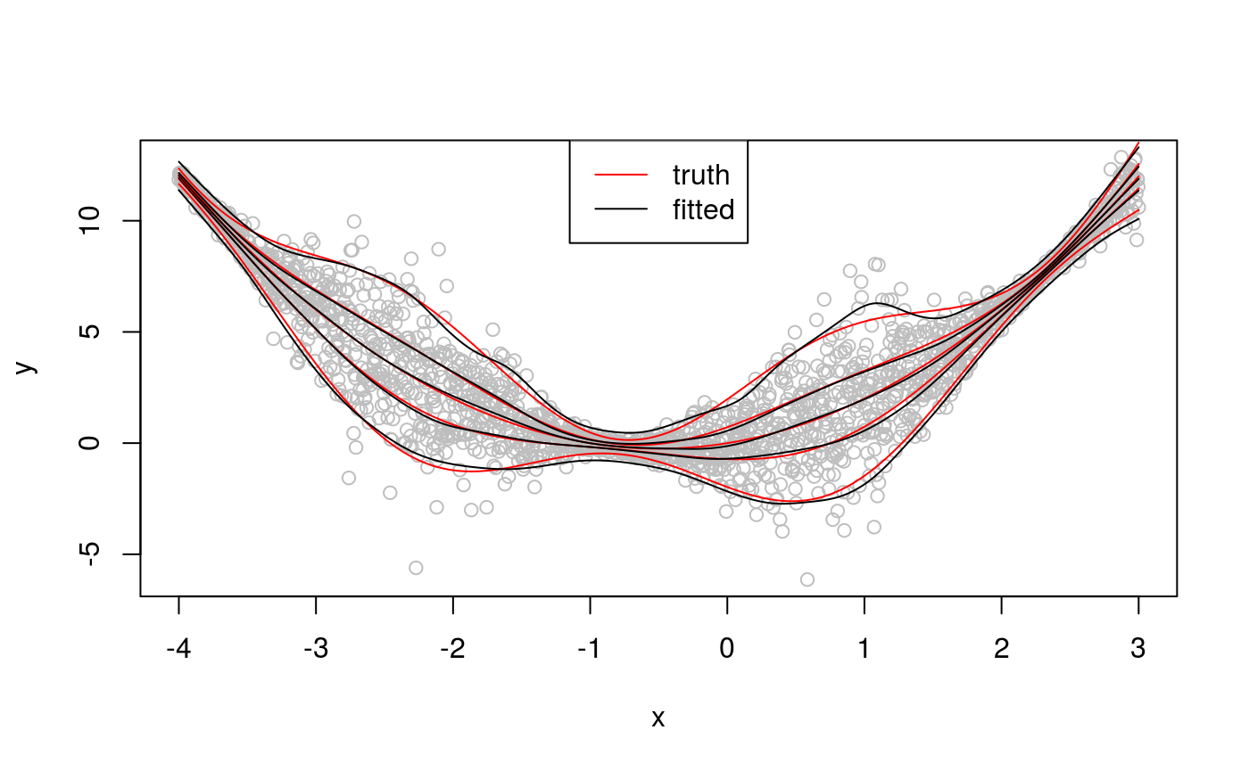

With the exception of qu = 0.95, the fitted quantiles are close to the true ones, but their credible intervals don’t vary much with x. Indeed, let’s look at intervals for quantile 0.95.

plot(x, dat, col = "grey", ylab = "y")
tmp <- qdo(fit, 0.95, predict, se = TRUE)
lines(x, tmp$fit)
lines(x, tmp$fit + 3 * tmp$se.fit, col = 2)
lines(x, tmp$fit - 3 * tmp$se.fit, col = 2)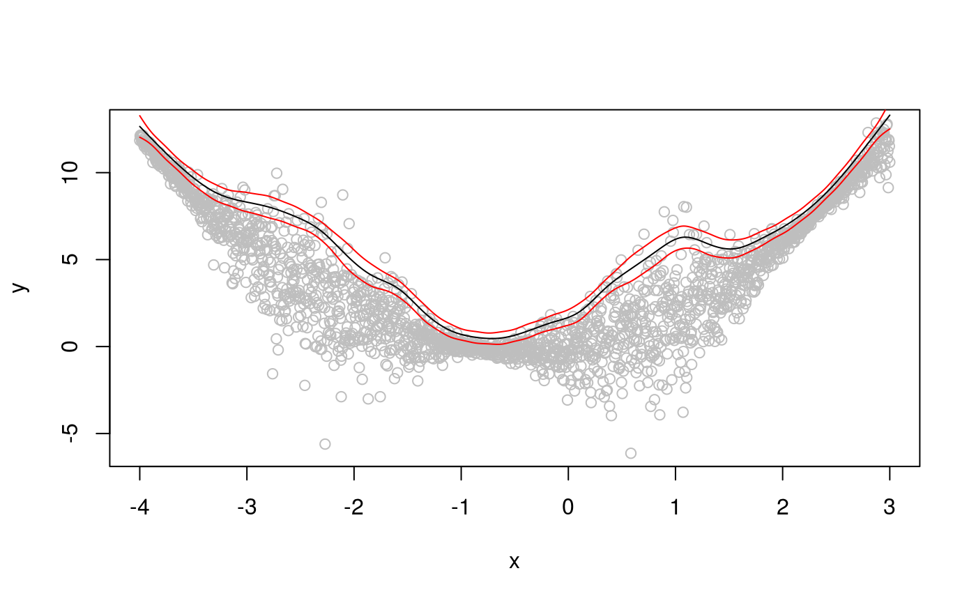

We can get better credible intervals, and solve the “wigglines” problem for the top quantile, by letting the learning rate vary with the covariate. In particular, we can use an additive model for quantile location and one for learning rate.

fit <- qgam(list(y~s(x, k = 30, bs = "cr"), ~ s(x, k = 30, bs = "cr")), 
            data = dataf, qu = 0.95)

## Estimating learning rate. Each dot corresponds to a loss evaluation. 
## qu = 0.95.........done

plot(x, dat, col = "grey", ylab = "y")
tmp <- predict(fit, se = TRUE)
lines(x, tmp$fit)
lines(x, tmp$fit + 3 * tmp$se.fit, col = 2)
lines(x, tmp$fit - 3 * tmp$se.fit, col = 2)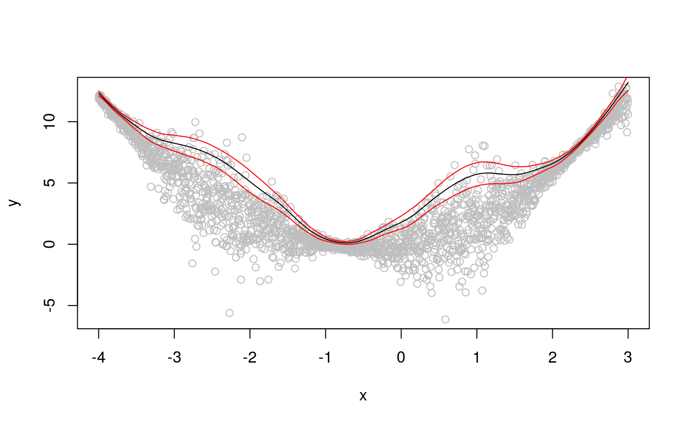

Now the credible intervals correctly represent the underlying uncertainty, and the fit has the correct amount of smoothness.

Neglecting to take the heteroscedasticity into account can lead to bias, in addition to inadequate coverage of the credible intervals. Let’s go back the motorcycle data set, and to the first model we fitted:

fit <- qgam(accel~s(times, k=20, bs="ad"), 
            data = mcycle, 
            qu = 0.8)

## Estimating learning rate. Each dot corresponds to a loss evaluation. 
## qu = 0.8............done

# Plot the fit
xSeq <- data.frame(cbind("accel" = rep(0, 1e3), "times" = seq(2, 58, length.out = 1e3)))
pred <- predict(fit, newdata = xSeq, se=TRUE)
plot(mcycle$times, mcycle$accel, xlab = "Times", ylab = "Acceleration", ylim = c(-150, 80))
lines(xSeq$times, pred$fit, lwd = 1)
lines(xSeq$times, pred$fit + 2*pred$se.fit, lwd = 1, col = 2)
lines(xSeq$times, pred$fit - 2*pred$se.fit, lwd = 1, col = 2)

The slightly disturbing thing about this quantile fit is that for Times < 10 the fit is clearly above all the responses. But we are fitting quantile 0.8, hence we should expect around 20$\%$ of the responses to be above the fit. The problem here is that the variance of the response (accel) varies wildly with Times, so that the bias induced by the smoothed pinball loss used by qgam is not constant (see Fasiolo et al. 2017 for details). This issue is solved by letting the learning rate change with Times:

fit <- qgam(list(accel ~ s(times, k=20, bs="ad"), ~ s(times)),
            data = mcycle, 
            qu = 0.8)

## Estimating learning rate. Each dot corresponds to a loss evaluation. 
## qu = 0.8................done

pred <- predict(fit, newdata = xSeq, se=TRUE)
plot(mcycle$times, mcycle$accel, xlab = "Times", ylab = "Acceleration", ylim = c(-150, 80))
lines(xSeq$times, pred$fit, lwd = 1)
lines(xSeq$times, pred$fit + 2*pred$se.fit, lwd = 1, col = 2)
lines(xSeq$times, pred$fit - 2*pred$se.fit, lwd = 1, col = 2)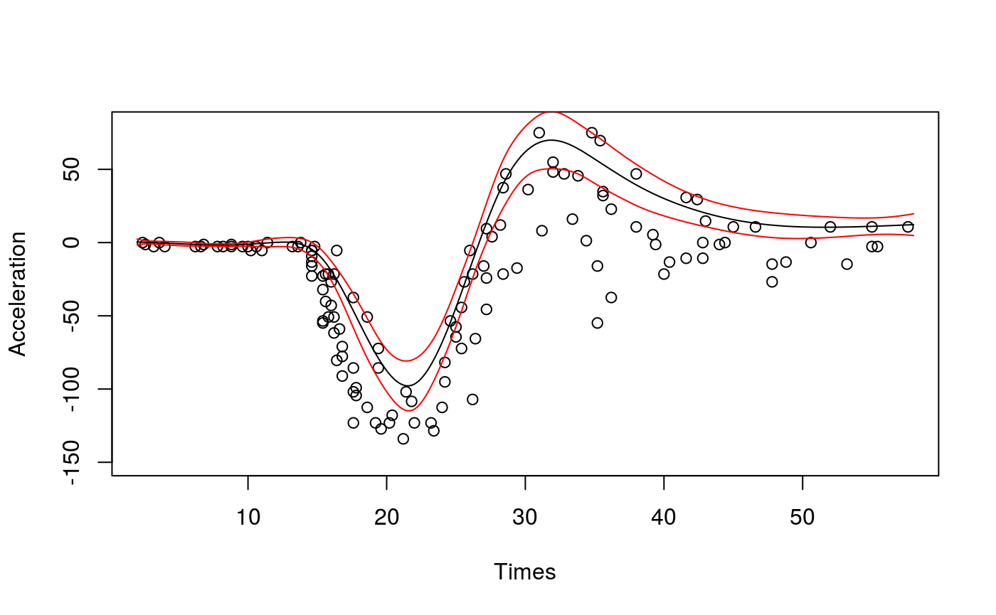

Model checking

The qgam package provides some functions that can be useful for model checking, but a more complete set of visualisation and checking tools can be found in the mgcViz R package (Fasiolo et al., 2018). In qgam we have:

cqcheck if we are fitting, say, quantile 0.2 we expect roughly $20\%$ of the observations to fall below the fitted quantile. This function produces some plots to verify this.
cqcheckI interactive version of cqcheckI. Implemented using the shiny package. Not demonstrated here, but see ?cqcheckI.
check.qgam provides some diagnostics regarding the optimization. Mainly based to gam.check.
check.learn diagnostic checks to verify that the learning rate selection went well. It can be used on the output of tuneLearn.
check.tuneLearn similar to check.learn, but it can be used on the output of tuneLearn or on the $calibr slot of a qgam object.

We start by illustrating the cqcheck function. In particular, let us consider the additive model: \[ y \sim x+x^2+z+xz/2+e,\;\;\; e \sim N(0, 1) \] We start by simulating some data from it.

library(qgam)
set.seed(15560)
n <- 1000
x <- rnorm(n, 0, 1); z <- rnorm(n)
X <- cbind(1, x, x^2, z, x*z)
beta <- c(0, 1, 1, 1, 0.5)
y <- drop(X %*% beta) + rnorm(n) 
dataf <- data.frame(cbind(y, x, z))
names(dataf) <- c("y", "x", "z")

We fit a linear model to the median and we use cqcheck produce a diagnostic plot.

qu <- 0.5
fit <- qgam(y~x, qu = qu, data = dataf)

## Estimating learning rate. Each dot corresponds to a loss evaluation. 
## qu = 0.5.........done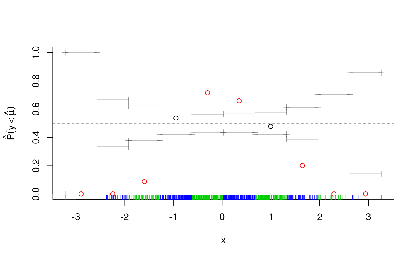

cqcheck(obj = fit, v = c("x"), X = dataf, y = y)

The cqcheck function takes a qgam object as input and it predicts the conditional quantile using the data in X. Then it bins the responses y using the corresponding values of v and it calculates, for every bin, what fraction of responses falls below the fitted quantile. Given that we are fitting the median, we would expect that around $50\%$ of the point falls below the fit. But, as the plot shows, this fraction varies widely along x. There is clearly a non-linear relation between the quantile location and x, hence we add a smooth for x.

fit <- qgam(y~s(x), qu = qu, data = dataf)

## Estimating learning rate. Each dot corresponds to a loss evaluation. 
## qu = 0.5........done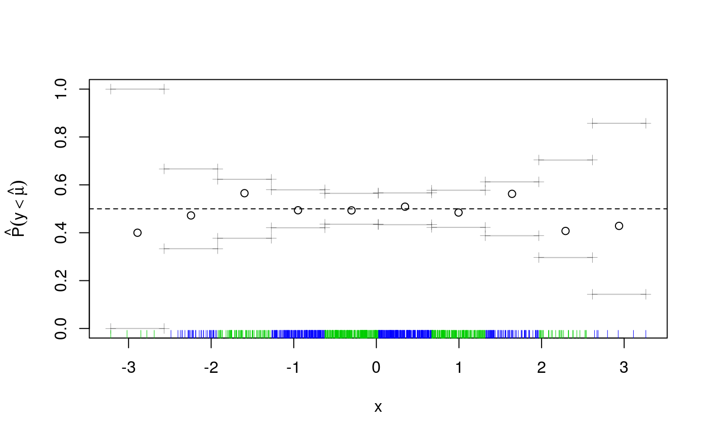

cqcheck(obj = fit, v = c("x"), X = dataf, y = y)

The deviations from the theoretical quantile ($0.5$) are much reduced, but let’s look across both x and z.

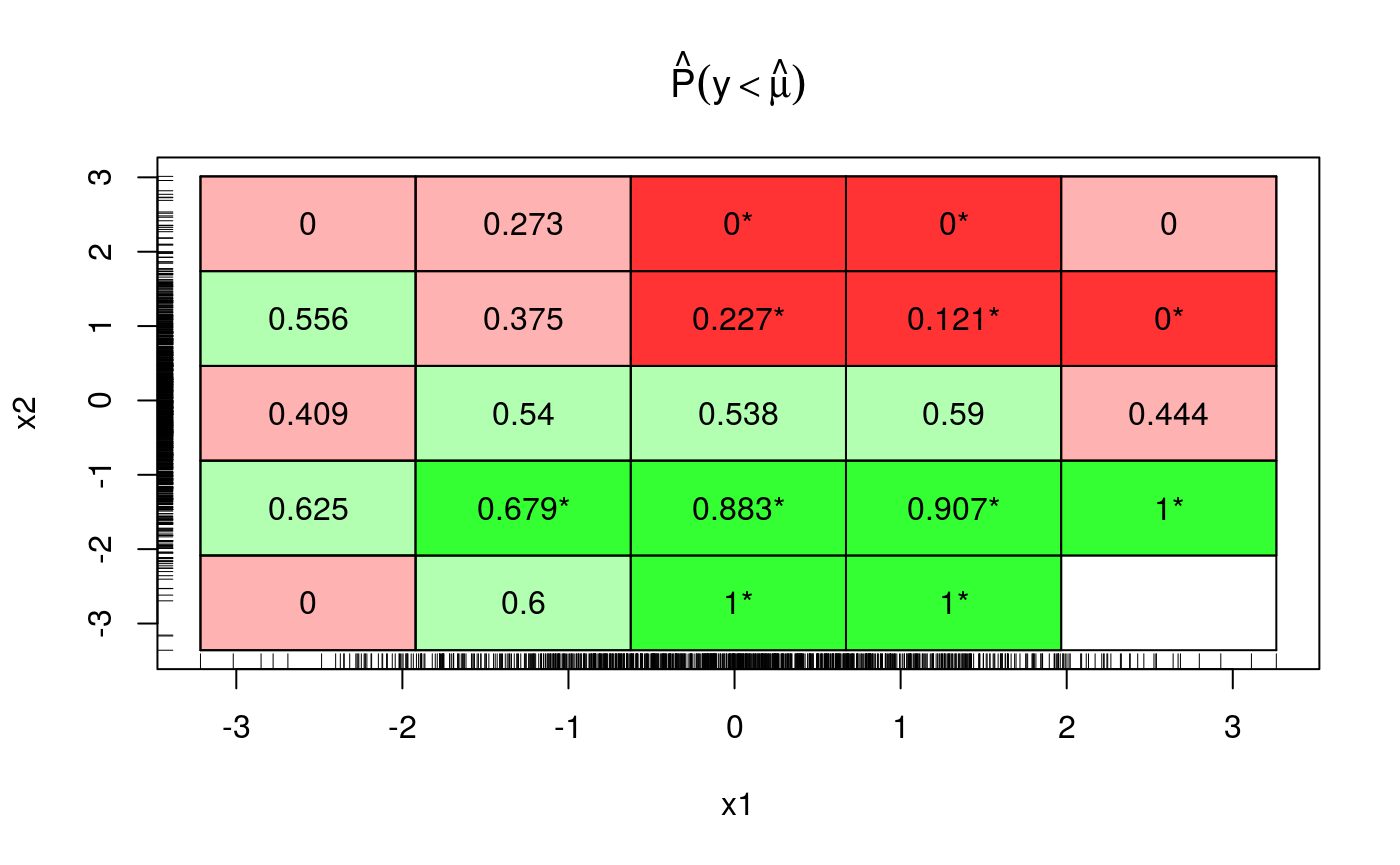
cqcheck(obj = fit, v = c("x", "z"), X = dataf, y = y, nbin = c(5, 5))

This plot uses binning as before, if a bin is red (green) this means that the fraction of responses falling below the fit is smaller (larger) than 0.5. Bright colours means that the deviation is statistically significant. As we move along z (x2 in the plot) the colour changes from green to red, so it make sense drawing a marginal plot for z:

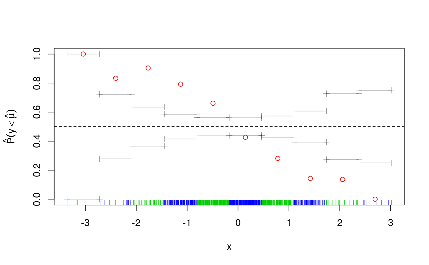
cqcheck(obj = fit, v = c("z"), X = dataf, y = y, nbin = c(10))

We are clearly missing an effect here. Given that effect looks pretty linear, we simply add a parametric term to the fit, which seems to solve the problem:

fit <- qgam(y~s(x)+z, qu = qu, data = dataf)

## Estimating learning rate. Each dot corresponds to a loss evaluation. 
## qu = 0.5.........done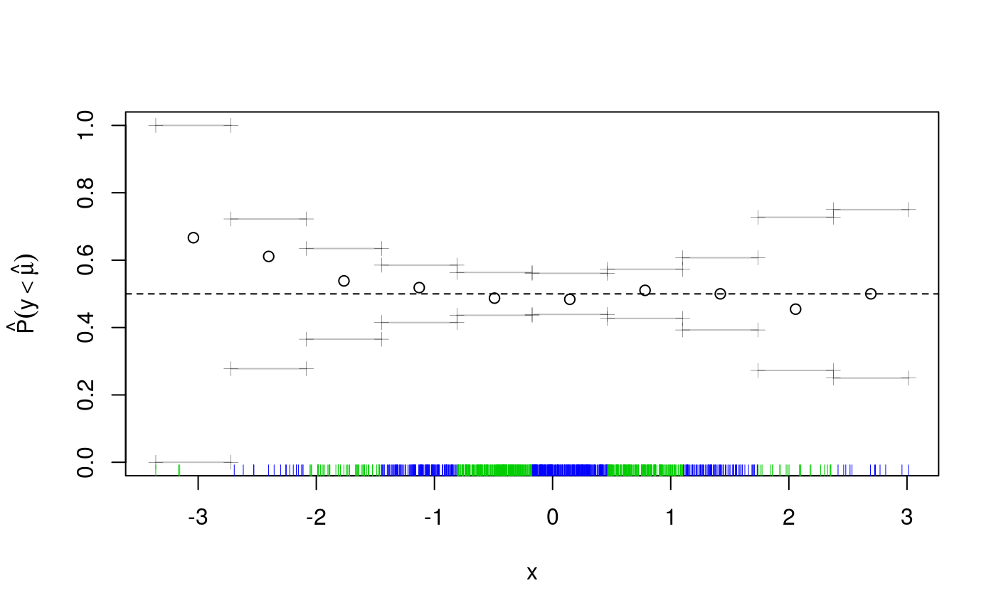

cqcheck(obj = fit, v = c("z"))

But if we look again across both x and z we see that green prevails on the top-left to bottom-right diagonal, while the other diagonal is mainly red.

cqcheck(obj = fit, v = c("x", "z"), nbin = c(5, 5))

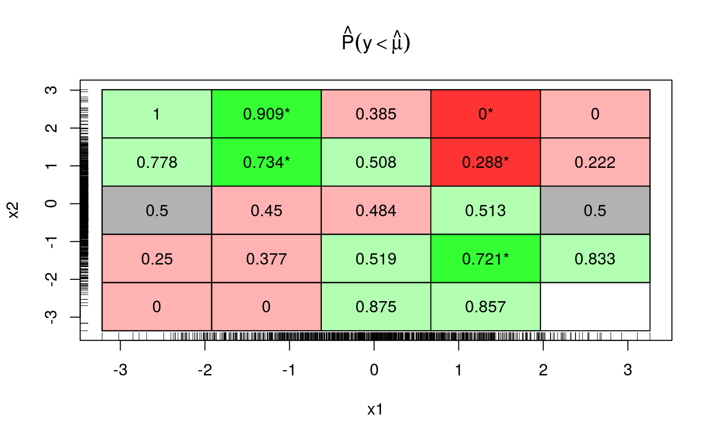
This suggests that adding an interaction between x and z might be a good idea. Indeed, now cqcheck does not signal any problem:

fit <- qgam(y~s(x)+z+I(x*z), qu = qu, data = dataf)

## Estimating learning rate. Each dot corresponds to a loss evaluation. 
## qu = 0.5........done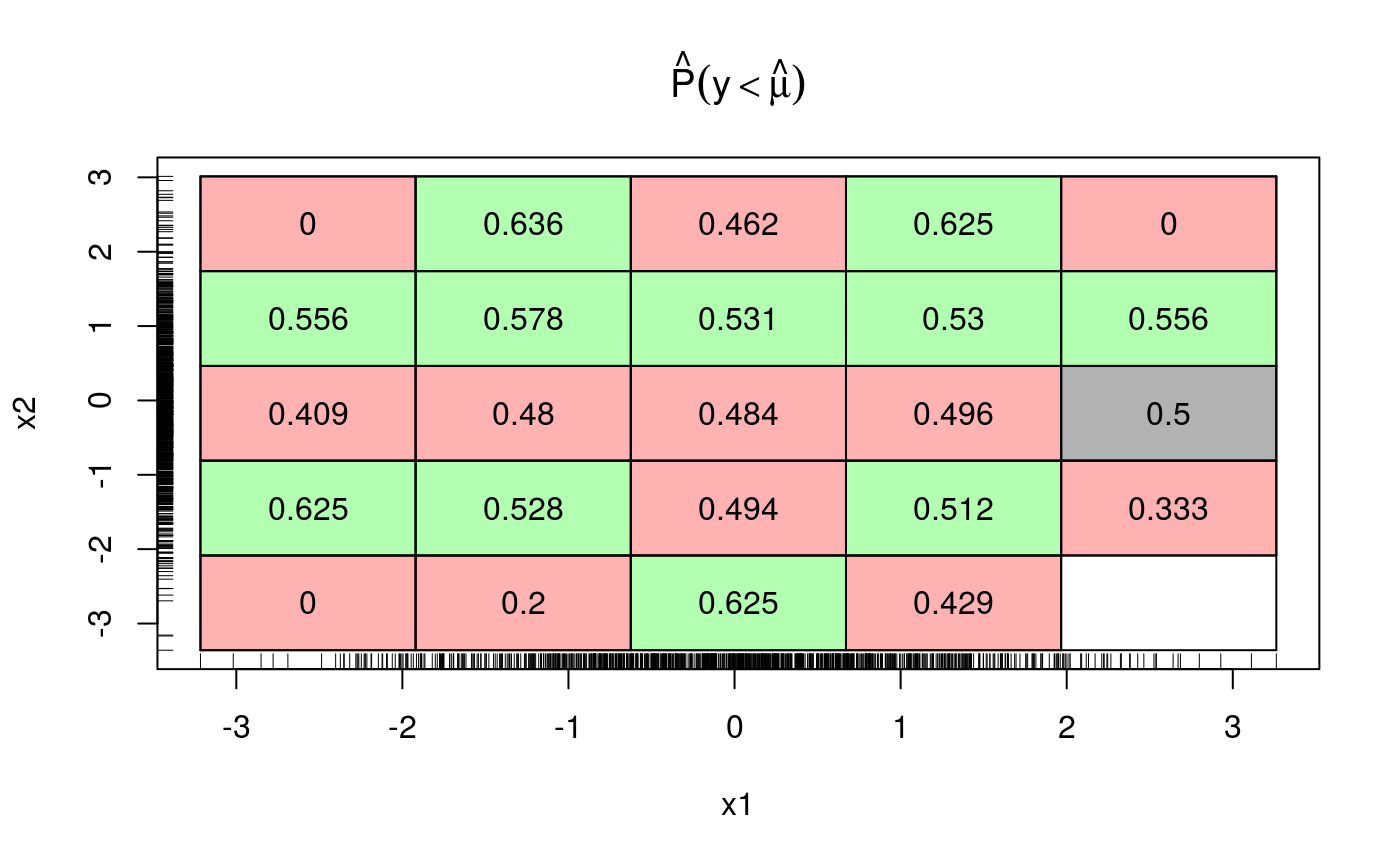

cqcheck(obj = fit, v = c("x", "z"), nbin = c(5, 5))

Now that we are fairly satisfied with the model structure, we can, for instance, fit several quantiles by doing:

fit <- mqgam(y~s(x)+z+I(x*z), qu = c(0.2, 0.4, 0.6, 0.8), data = dataf)

## Estimating learning rate. Each dot corresponds to a loss evaluation. 
## qu = 0.4........done 
## qu = 0.6.........done 
## qu = 0.2.......done 
## qu = 0.8...............done

We can then check whether the learning rate was selected correctly. Recall that the qgam function calls internally tuneLearnFast, hence we can look at how the calibration went by doing:

check.learnFast(fit$calibr, 2:5)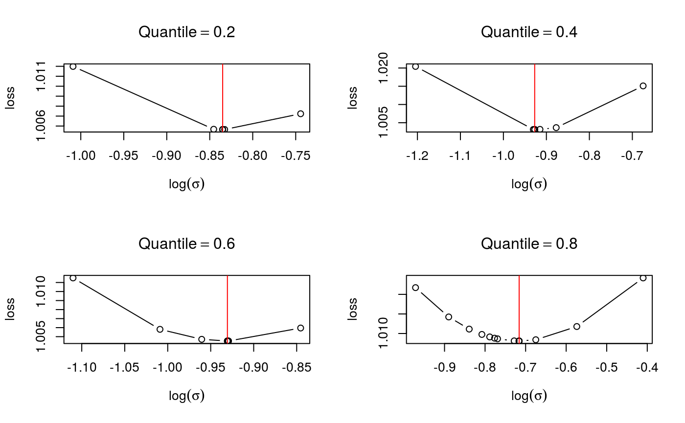

For each quantile, the calibration loss seems to have a unique minimum, which is what one would hope. Objects of class qgam can also be checked using the generic function check, which defaults to check.qgam. To use this function on the output of mqgam, we must use the qdo function:

qdo(fit, 0.2, check)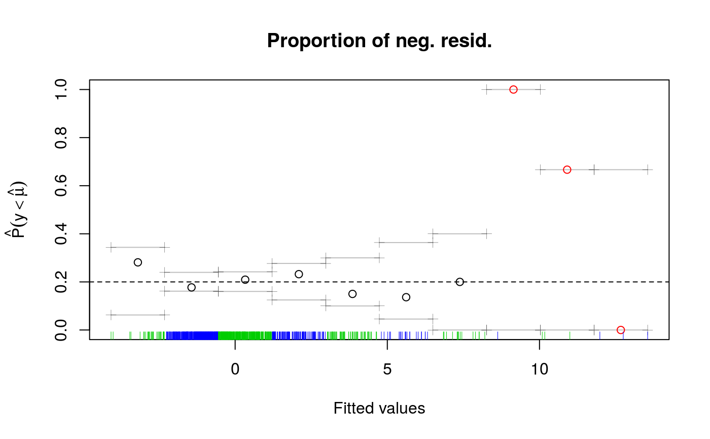

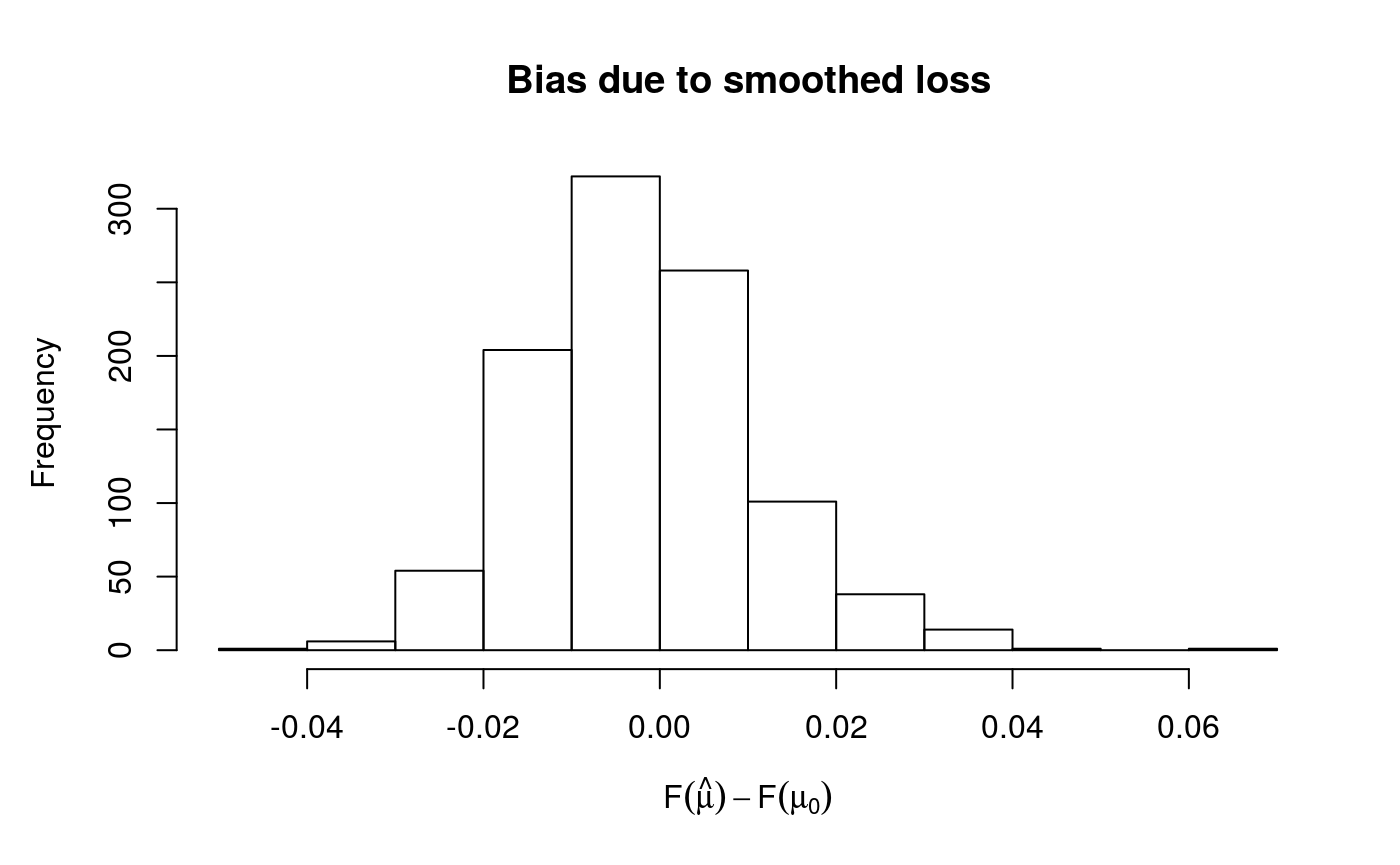
## Theor. proportion of neg. resid.: 0.2   Actual proportion: 0.198
## Integrated absolute bias |F(mu) - F(mu0)| = 0.01025554
## Method: REML   Optimizer: outer newton
## full convergence after 4 iterations.
## Gradient range [0.00075606,0.00075606]
## (score 1658.424 & scale 1).
## Hessian positive definite, eigenvalue range [3.83483,3.83483].
## Model rank =  12 / 12 
## 
## Basis dimension (k) check: if edf is close too k' (maximum possible edf) 
## it might be worth increasing k. 
## 
##      k'  edf
## s(x)  9 7.38

## NULL

The printed output gives some information about the optimizer used to estimate the smoothing parameters, for fixed learning rate. See ?check.qgam for more information. The plot has been obtained using cqcheck, where each data point has been binned using the fitted values. On the right side of the plot there seems to be some large deviations, but the rug shows that there are very few data points there.

Setting the loss-smoothing parameter and checking convergence

Let’s simulate some data:

set.seed(5235)
n <- 1000
x <- seq(-3, 3, length.out = n)
X <- cbind(1, x, x^2)
beta <- c(0, 1, 1)
f <- drop(X %*% beta)
dat <- f + rgamma(n, 4, 1)
dataf <- data.frame(cbind(dat, x))
names(dataf) <- c("y", "x")

Assume that we want to estimate quantiles 0.05, 0.5 and 0.95:

qus <- c(0.05, 0.5, 0.95)
fit <- mqgam(y ~ s(x), data = dataf, qu = qus)

## Estimating learning rate. Each dot corresponds to a loss evaluation. 
## qu = 0.5........done 
## qu = 0.95........done 
## qu = 0.05.................done

plot(x, dat, col = "grey", ylab = "y")
lines(x, f + qgamma(0.95, 4, 1), lty = 2)
lines(x, f + qgamma(0.5, 4, 1), lty = 2)
lines(x, f + qgamma(0.05, 4, 1), lty = 2)
lines(x, qdo(fit, qus[1], predict), col = 2)
lines(x, qdo(fit, qus[2], predict), col = 2)
lines(x, qdo(fit, qus[3], predict), col = 2)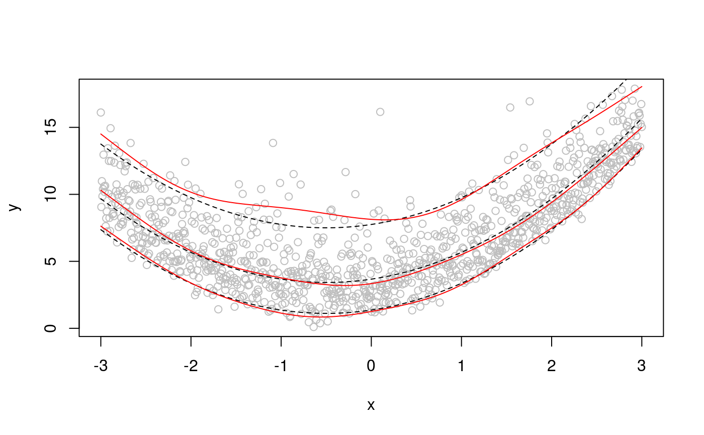

Since qgam version 1.3 the parameter err, which determines the smoothness of the loss function used by qgam, is determined automatically. But there might be scenarios where you might want to chose is manually, so let’s try to use several values of err:

lfit <- lapply(c(0.01, 0.05, 0.1, 0.2, 0.3, 0.5),
               function(.inp){
                 mqgam(y ~ s(x), data = dataf, qu = qus, err = .inp, 
                       control = list("progress" = F))
               })

plot(x, dat, col = "grey", ylab = "y", ylim = c(-2, 20))
colss <- rainbow(length(lfit))
for(ii in 1:length(lfit)){
  lines(x, qdo(lfit[[ii]], qus[1], predict), col = colss[ii])
  lines(x, qdo(lfit[[ii]], qus[2], predict), col = colss[ii])
  lines(x, qdo(lfit[[ii]], qus[3], predict), col = colss[ii])
}
lines(x, f + qgamma(0.95, 4, 1), lty = 2)
lines(x, f + qgamma(0.5, 4, 1), lty = 2)
lines(x, f + qgamma(0.05, 4, 1), lty = 2)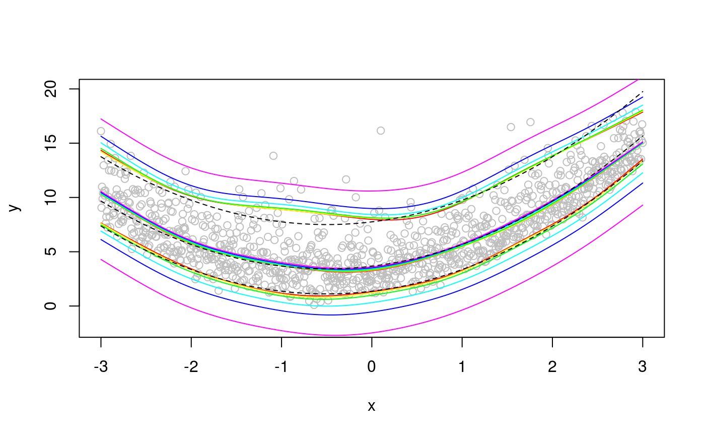

The bias increases with err, and it is upward (downward) for high (low) quantiles. The median fit is not much affected by err. The bias really starts appearing for err > 0.1. Decreasing err tends to slow down computation:

system.time( fit1 <- qgam(y ~ s(x), data = dataf, qu = 0.95, err = 0.05, 
                           control = list("progress" = F)) )[[3]]

## [1] 0.264

system.time( fit2 <- qgam(y ~ s(x), data = dataf, qu = 0.95, err = 0.001, 
                           control = list("progress" = F)) )[[3]]

## [1] 27.455

Even worse, it can lead to numeric problems. Here we check that we have found the minimum of the calibration loss:

check(fit1$calibr, sel = 2)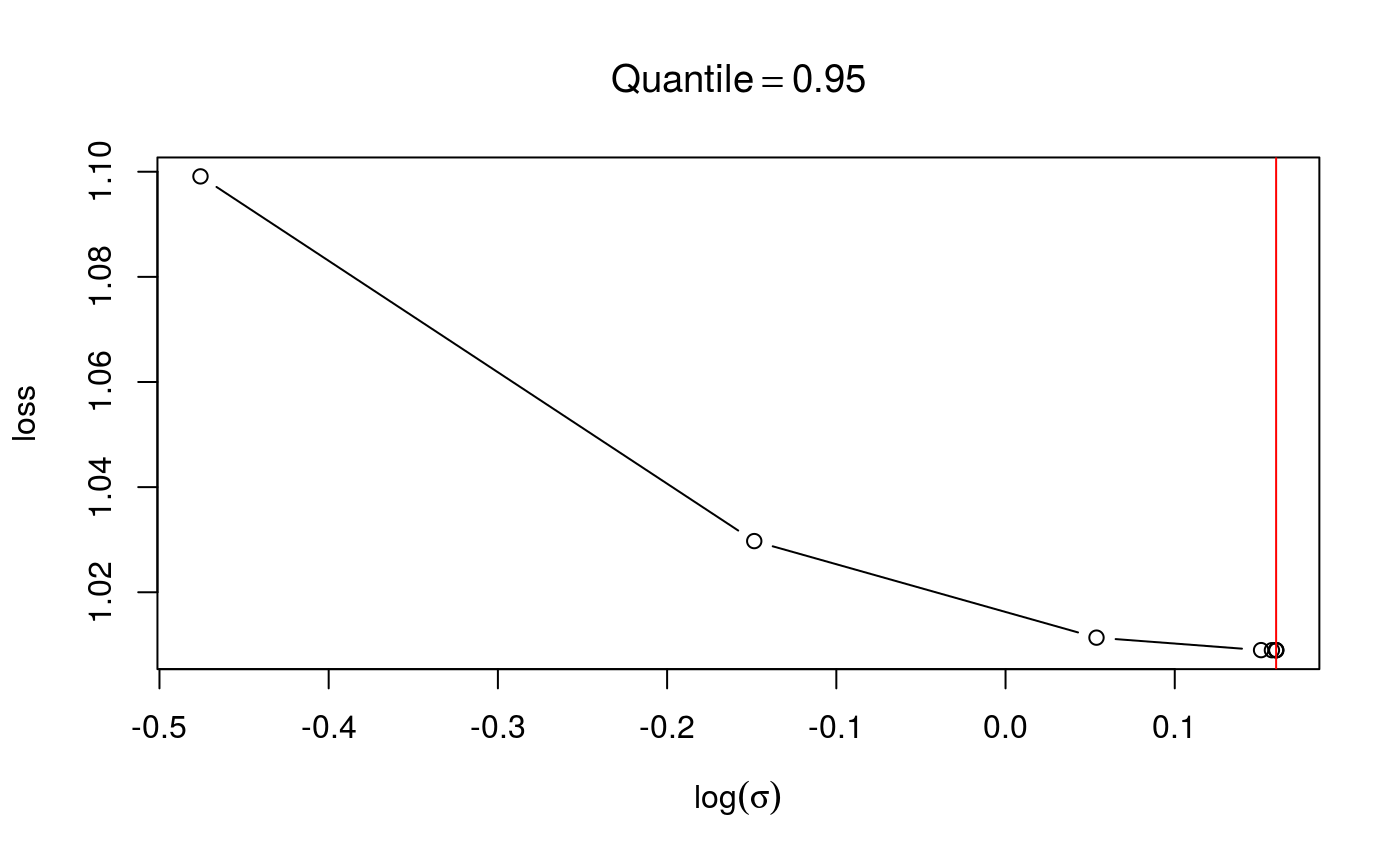

check(fit2$calibr, sel = 2)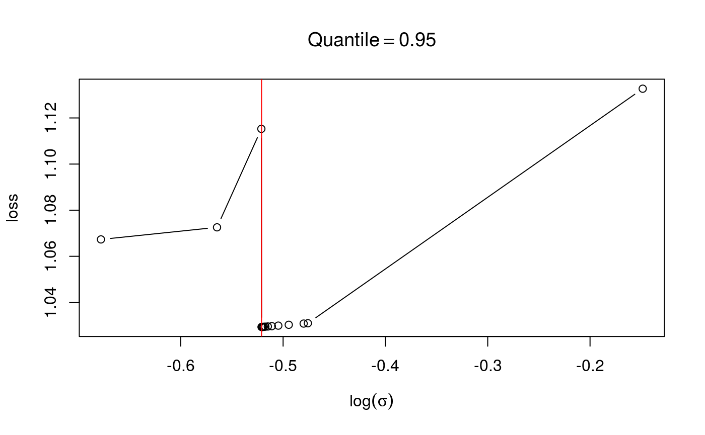

In the first case the loss looks smooth and with as single minimum, in the second case we have some instabilities. If the calibration loss looks like this, you generally have to increase err.

We can use check to have an estimate of the bias and to have information regarding the convergence of the smoothing parameter estimation routine:

check(fit1)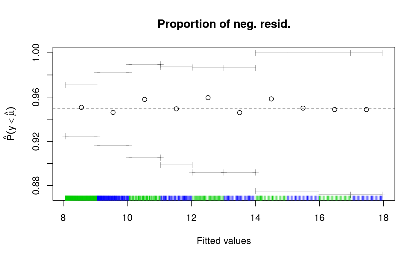

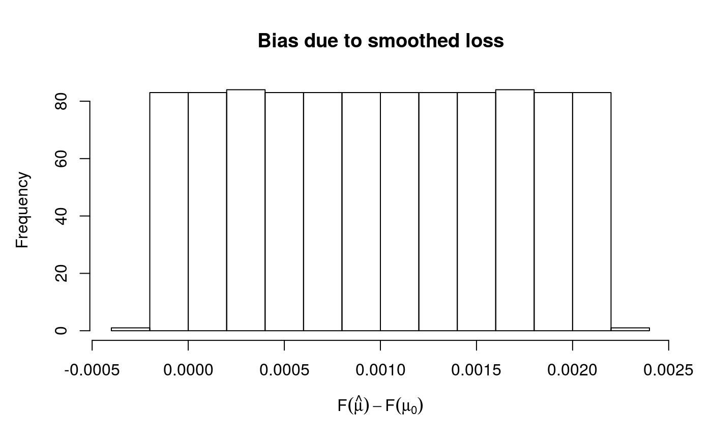
## Theor. proportion of neg. resid.: 0.95   Actual proportion: 0.951
## Integrated absolute bias |F(mu) - F(mu0)| = 0.001017127
## Method: REML   Optimizer: outer newton
## full convergence after 5 iterations.
## Gradient range [4.449524e-08,4.449524e-08]
## (score 3438.722 & scale 1).
## Hessian positive definite, eigenvalue range [1.428662,1.428662].
## Model rank =  10 / 10 
## 
## Basis dimension (k) check: if edf is close too k' (maximum possible edf) 
## it might be worth increasing k. 
## 
##      k'  edf
## s(x)  9 5.05

The second plot suggest that the actual bias is much lower than the bound err = 0.05. This is also supported by the first two lines of text, which say that 95.1% of the residuals are negative, which is very close to the theoretical 95%. The text says that full convergence in smoothing parameter estimation has been achieved, it is important to check this.

In summary, practical experience suggests that:

the automatic procedure for selecting err offer a good compromise between bias and stability;
the old default (qgam version < 1.3) was err = 0.05, which generally does not imply too much bias;
if the calibration loss plotted by check(fit$learn) is irregular, try to increase err;
same if the text printed by check(fit) does not say that full convergence was achieved;
you can estimate the bias using check(fit);
if you have to increase err to 0.2 or higher, there might be something wrong with your model;
you might get messages saying that outer Newton did not converge fully during estimation. This might not be problematic as long as the calibration loss is smooth and full convergence was achieved;
in preliminary studies do not decrease err too much, as it slows down computation;
setting err too low is not a good idea: it is much better to have some bias than numerical problems.

Application to probabilistic electricity load forecasting

Here we consider a UK electricity demand dataset, taken from the national grid website. The dataset covers the period January 2011 to June 2016 and it contains the following variables:

NetDemand net electricity demand between 11:30am and 12am.
wM instantaneous temperature, averaged over several English cities.
wM_s95 exponential smooth of wM, that is wM_s95[i] = a*wM[i] + (1-a)*wM_s95[i] with a=0.95.
Posan periodic index in [0, 1] indicating the position along the year.
Dow factor variable indicating the day of the week.
Trend progressive counter, useful for defining the long term trend.
NetDemand.48 lagged version of NetDemand, that is NetDemand.48[i] = NetDemand[i-2].
Holy binary variable indicating holidays.
Year and Date should obvious, and partially redundant.

See Fasiolo et al., 2017 for more details. This is how the demand over the period looks like:

data("UKload")
tmpx <- seq(UKload$Year[1], tail(UKload$Year, 1), length.out = nrow(UKload)) 
plot(tmpx, UKload$NetDemand, type = 'l', xlab = 'Year', ylab = 'Load')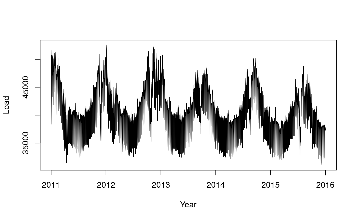

To estimate the median demand, we consider the following model

qu <- 0.5
form <- NetDemand~s(wM,k=20,bs='cr') + s(wM_s95,k=20,bs='cr') + 
        s(Posan,bs='ad',k=30,xt=list("bs"="cc")) + Dow + s(Trend,k=4) + NetDemand.48 + Holy

Notice that we use very few knots for the long term trend, this is because we don’t want to end up interpolating the data. We use an adaptive cyclic smooth for Posan, we’ll explain later why adaptivity is needed here.

Now we tune the learning rate on a grid, on two cores. As the first plot shows, the calibrations loss is minimized at $\log (\sigma)\approx 6$, the second plot shows how the effective degrees of freedom of each smooth term changes with $\log (\sigma)$.

set.seed(41241)
sigSeq <- seq(4, 8, length.out = 16)
closs <- tuneLearn(form = form, data = UKload, 
                   lsig = sigSeq, qu = qu, control = list("K" = 20), 
                   multicore = TRUE, ncores = 2)

check(closs)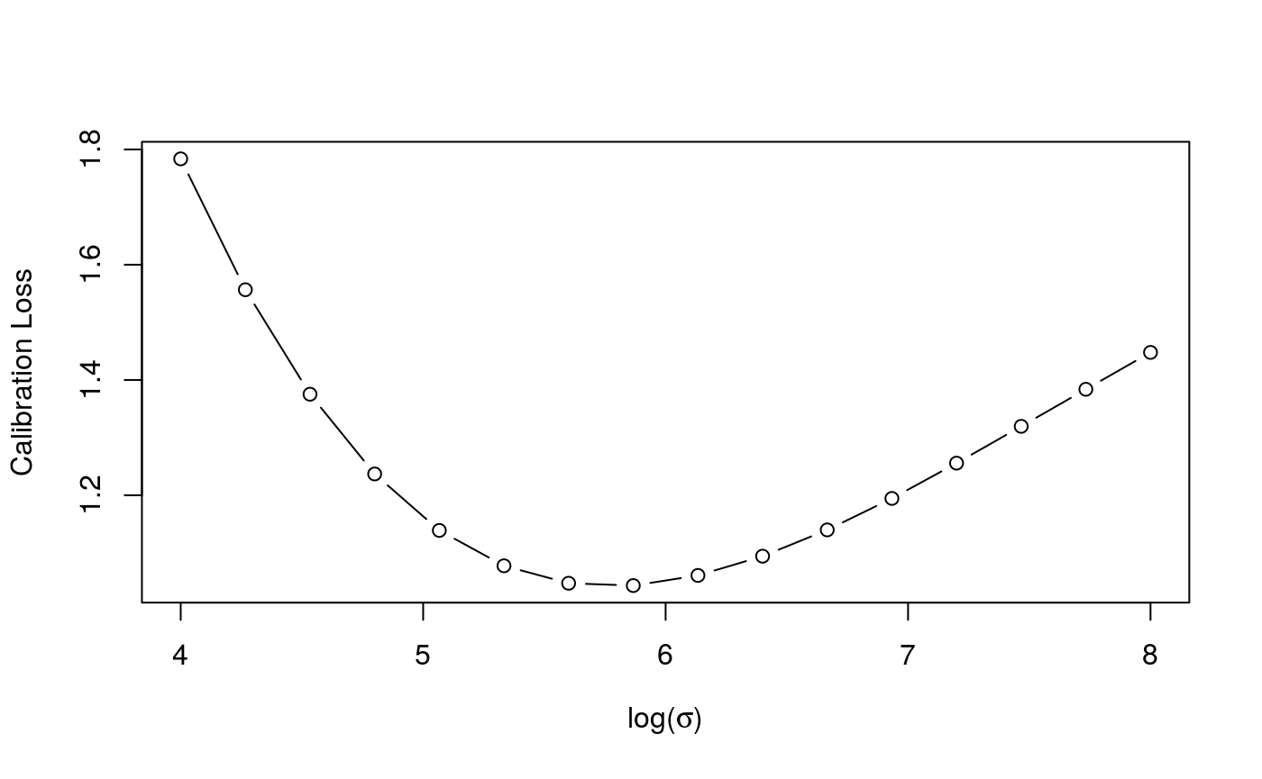

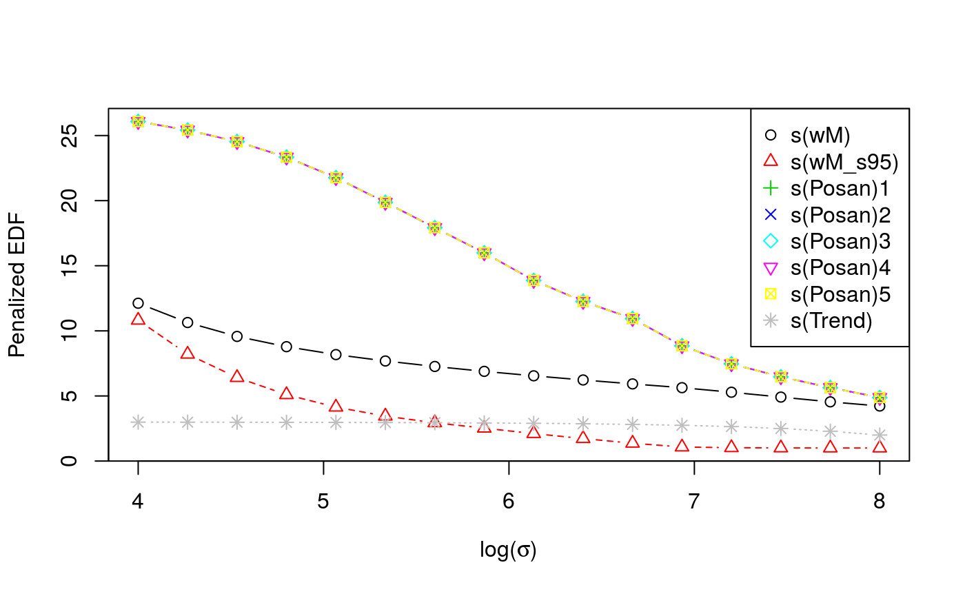
Now let’s fit the model with the learning rate corresponding to the lowest loss and let’s look at the resulting smooth effects.

lsig <- closs$lsig
fit <- qgam(form = form, data = UKload, lsig = lsig, qu = qu)
plot(fit, scale = F, page = 1)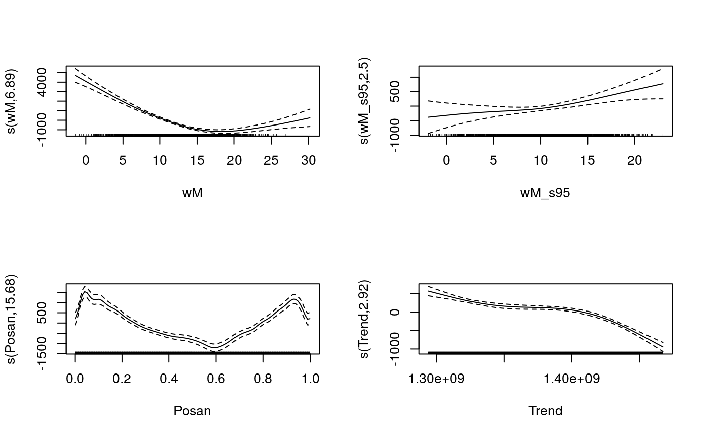

The effect of temperature (wM) is minimized around 18 degrees, which is reasonable. The cyclic effect of Posan has a very sharp drop corresponding to the winter holidays, we used an adaptive smooth in order to have more flexibility during this period. Now we can have a look as some diagnostic plot:

par(mfrow = c(2, 2))
cqcheck(fit, v = c("wM"), main = "wM")
cqcheck(fit, v = c("wM_s95"), main = "wM_s95")
cqcheck(fit, v = c("Posan"), main = "Posan")
cqcheck(fit, v = c("Trend"), main = "Trend", xaxt='n')
axis(1, at = UKload$Trend[c(1, 500, 1000, 1500, 2000)], 
             UKload$Year[c(1, 500, 1000, 1500, 2000)] )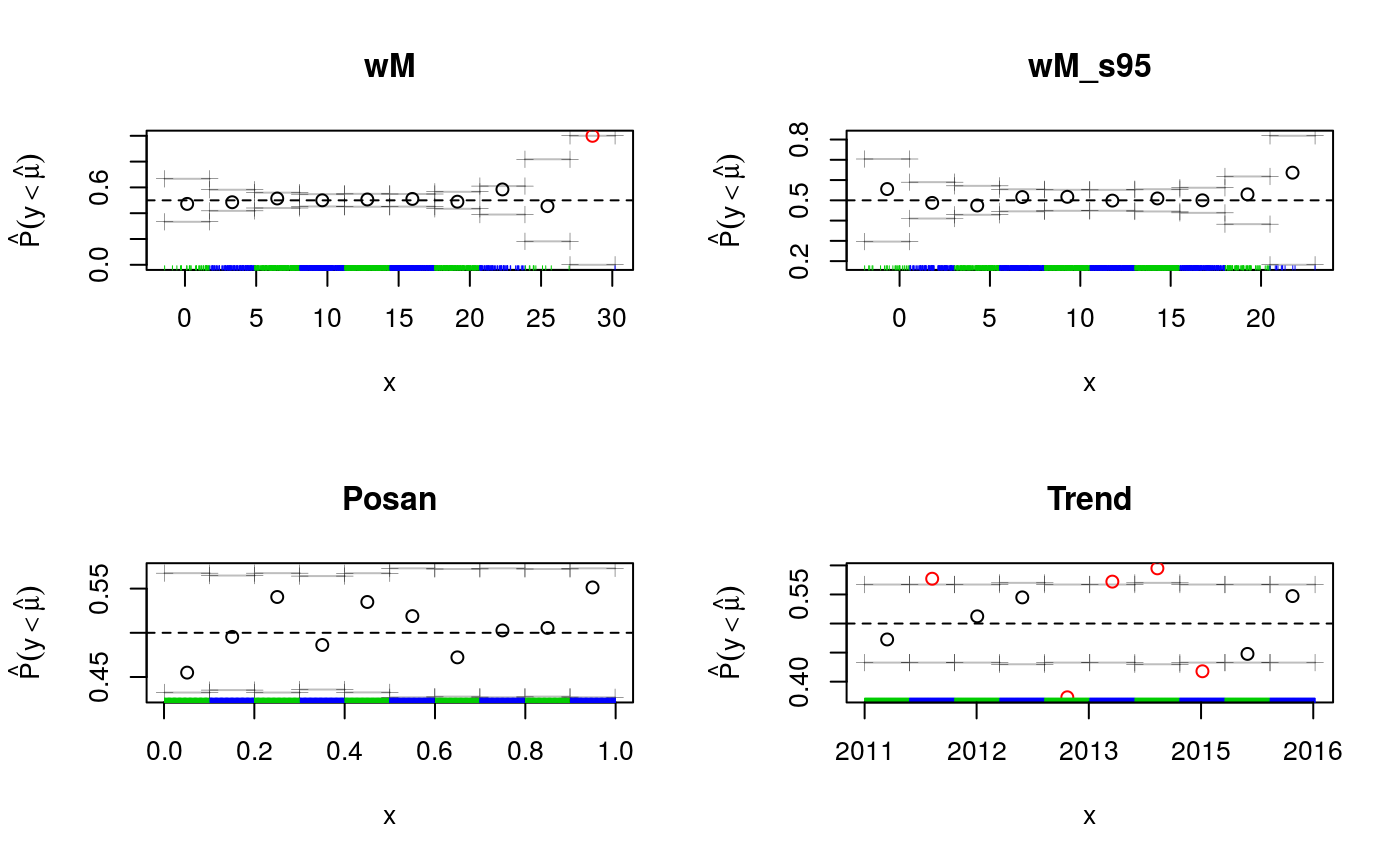

The plots for wM_s95 and Posan don’t show any important deviation from 0.5, the target quantile. Along wM we see a large deviation, but we have essentially no data for very high temperatures. If we look at deviations along the Trend variable, which is just a time counter, we see several important deviations. It would be interesting verifying why these occur (we have no answer currently).

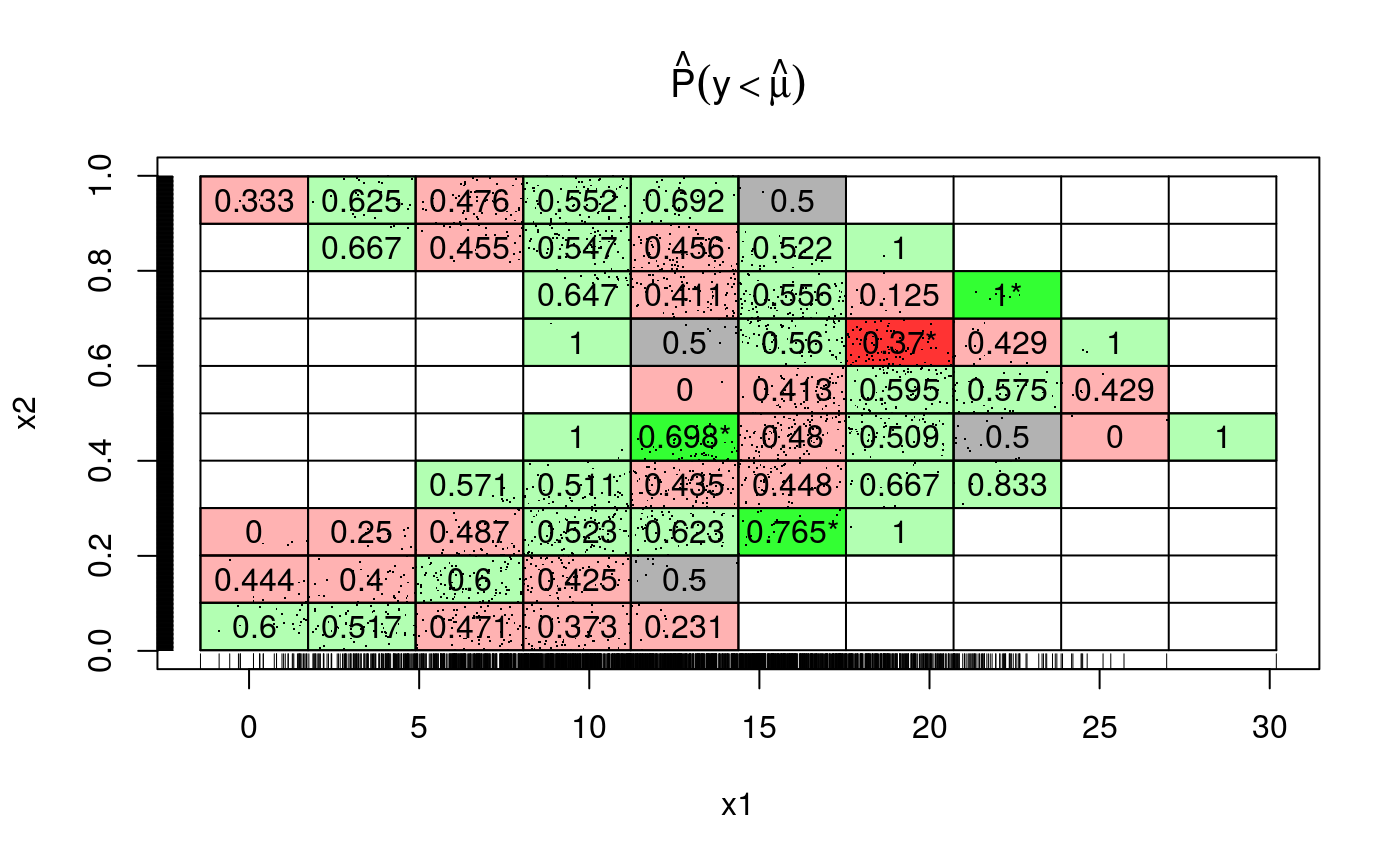
Finally, recall that we can produce 2D versions of these diagnostic plots, for instance:

par(mfrow = c(1, 1))
cqcheck(fit, v = c("wM", "Posan"), scatter = T)

References

Fasiolo, M., Goude, Y., Nedellec, R. and Wood, S. N. (2017). Fast calibrated additive quantile regression. Available at https://arxiv.org/abs/1707.03307
Fasiolo, M., Nedellec, R., Goude, Y. and Wood, S.N. (2018). Scalable visualisation methods for modern Generalized Additive Models. Available at https://arxiv.org/abs/1809.10632

qgam: quantile non-parametric additive models

Matteo Fasiolo, Simon N. Wood, Yannig Goude, and Raphael Nedellec