Fast learning rate calibration for the Gibbs posterior

The learning rate (sigma) of the Gibbs posterior is tuned either by calibrating the credible intervals for the fitted curve, or by minimizing the pinball loss on out-of-sample data. This is done by bootrapping or by k-fold cross-validation. Here the loss function is minimized, for each quantile, using a Brent search.

tuneLearnFast(form, data, qu, err = NULL,
  multicore = !is.null(cluster), cluster = NULL,
  ncores = detectCores() - 1, paropts = list(), control = list(),
  argGam = NULL)

Arguments

form	A GAM formula, or a list of formulae. See ?mgcv::gam details.
data	A data frame or list containing the model response variable and covariates required by the formula. By default the variables are taken from environment(formula): typically the environment from which gam is called.
qu	The quantile of interest. Should be in (0, 1).
err	An upper bound on the error of the estimated quantile curve. Should be in (0, 1). Since qgam v1.3 it is selected automatically, using the methods of Fasiolo et al. (2017). The old default was err=0.05.
multicore	If TRUE the calibration will happen in parallel.
cluster	An object of class c("SOCKcluster", "cluster"). This allowes the user to pass her own cluster, which will be used if multicore == TRUE. The user has to remember to stop the cluster.
ncores	Number of cores used. Relevant if multicore == TRUE.
paropts	a list of additional options passed into the foreach function when parallel computation is enabled. This is important if (for example) your code relies on external data or packages: use the .export and .packages arguments to supply them so that all cluster nodes have the correct environment set up for computing.
control	A list of control parameters for tuneLearn with entries: loss = loss function use to tune log(sigma). If loss=="cal" is chosen, then log(sigma) is chosen so that credible intervals for the fitted curve are calibrated. See Fasiolo et al. (2017) for details. If loss=="pin" then log(sigma) approximately minimizes the pinball loss on the out-of-sample data. sam = sampling scheme use: sam=="boot" corresponds to bootstrapping and sam=="kfold" to k-fold cross-validation. The second option can be used only if ctrl$loss=="pin". vtype = type of variance estimator used to standardize the deviation from the main fit in the calibration. If set to "m" the variance estimate obtained by the full data fit is used, if set to "b" than the variance estimated produced by the bootstrap fits are used. By default vtype="m". epsB = positive tolerance used to assess convergence when fitting the regression coefficients on bootstrap data. In particular, if |dev-dev_old|/(|dev|+0.1)<epsB then convergence is achieved. Default is epsB=1e-5. K = if sam=="boot" this is the number of boostrap datasets, while if sam=="kfold" this is the number of folds. By default K=50. init = an initial value for the log learning rate (log(sigma)). By default init=NULL and the optimization is initialized by other means. brac = initial bracket for Brent method. By default brac=log(c(0.5, 2)), so the initial search range is (init + log(0.5), init + log(2)). tol = tolerance used in the Brent search. By default tol=.Machine$double.eps^0.25. See ?optimize for details. aTol = Brent search parameter. If the solution to a Brent get closer than aTol * abs(diff(brac)) to one of the extremes of the bracket, the optimization is stop and restarted with an enlarged and shifted bracket. aTol=0.05 should be > 0 and values > 0.1 don't quite make sense. By default aTol=0.05. redWd = parameter which determines when the bracket will be reduced. If redWd==10 then the bracket is halved if the nearest solution falls within the central 10% of the bracket's width. By default redWd = 10. b = offset parameter used by the mgcv::gauslss, which we estimate to initialize the quantile fit (when a variance model is used). By default b=0. link = Link function to be used. See ?elf and ?elflss for defaults. verbose = if TRUE some more details are given. By default verbose=FALSE. progress = if TRUE progress in learning rate estimation is reported via printed text. TRUE by default.
argGam	A list of parameters to be passed to mgcv::gam. This list can potentially include all the arguments listed in ?gam, with the exception of formula, family and data.

Value

A list with entries:

• lsig = a vector containing the values of log(sigma) that minimize the loss function, for each quantile.

• err = the error bound used for each quantile. Generally each entry is identical to the argument err, but in some cases the function increases it to enhance stabily.

• ranges = the search ranges by the Brent algorithm to find log-sigma, for each quantile.

• store = a list, where the i-th entry is a matrix containing all the locations (1st row) at which the loss function has been evaluated and its value (2nd row), for the i-th quantile.

References

Fasiolo, M., Goude, Y., Nedellec, R. and Wood, S. N. (2017). Fast calibrated additive quantile regression. Available at https://arxiv.org/abs/1707.03307.

Examples

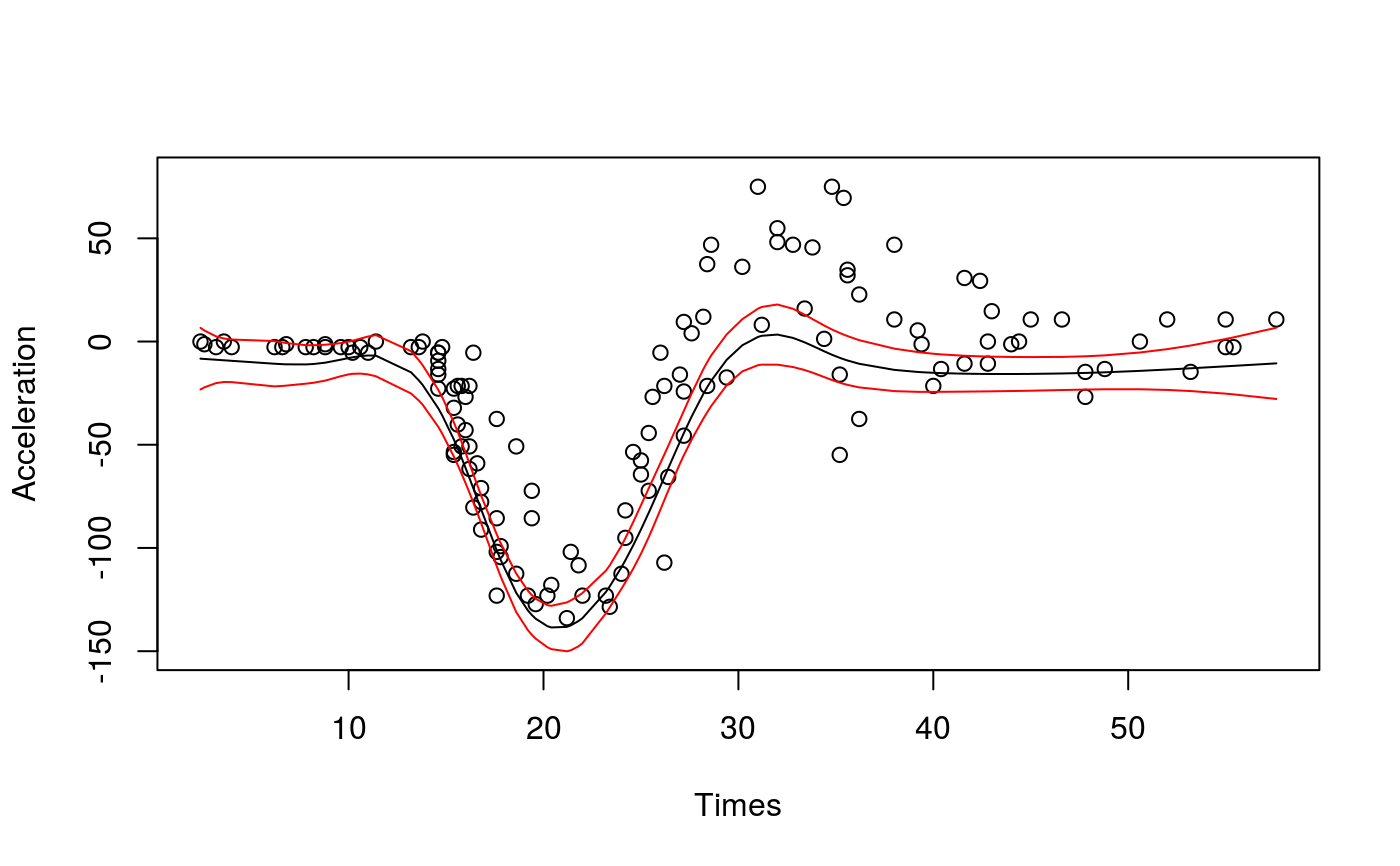
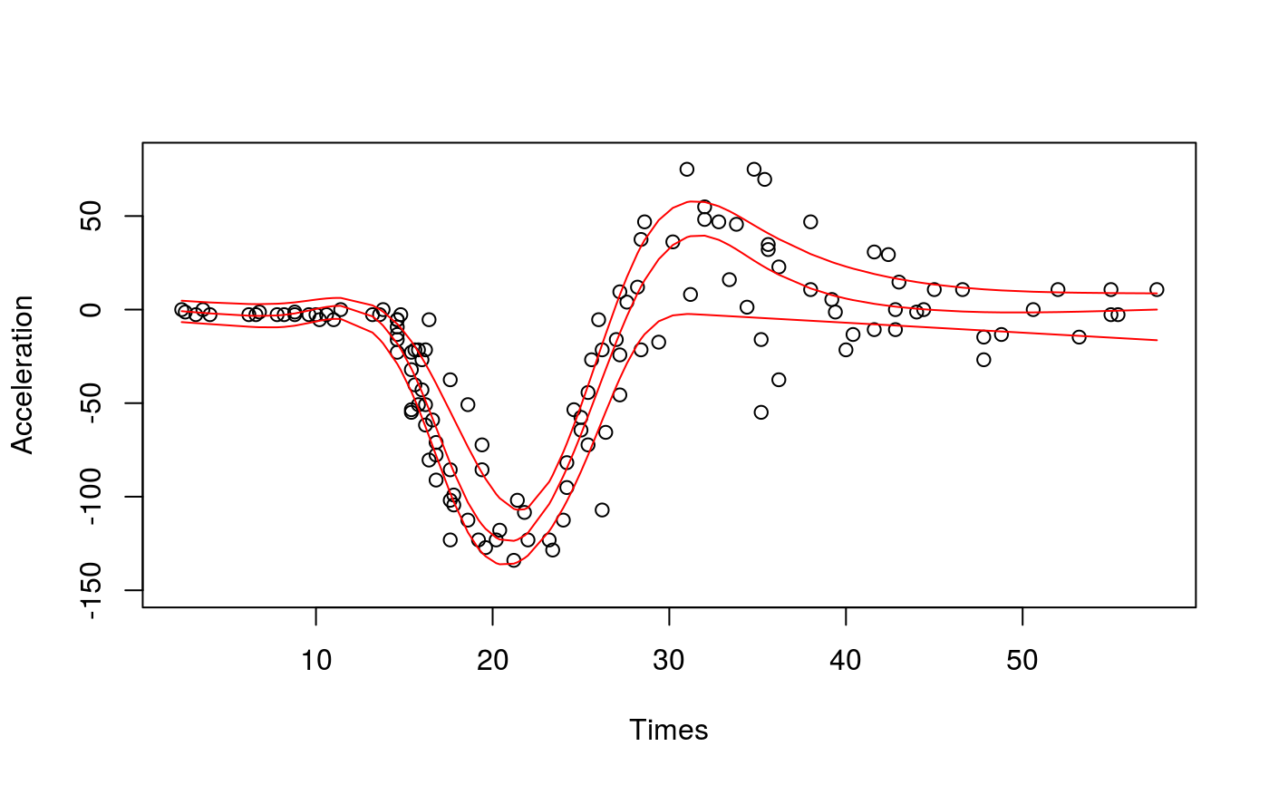
library(qgam); library(MASS)

###
# Single quantile fit
###
# Calibrate learning rate on a grid
set.seed(5235)
tun <- tuneLearnFast(form = accel~s(times,k=20,bs="ad"),
                     data = mcycle,
                     qu = 0.2)
#> Estimating learning rate. Each dot corresponds to a loss evaluation. 
#> qu = 0.2...........done 

# Fit for quantile 0.2 using the best sigma
fit <- qgam(accel~s(times, k=20, bs="ad"), data = mcycle, qu = 0.2, lsig = tun$lsig)

pred <- predict(fit, se=TRUE)
plot(mcycle$times, mcycle$accel, xlab = "Times", ylab = "Acceleration",
     ylim = c(-150, 80))
lines(mcycle$times, pred$fit, lwd = 1)
lines(mcycle$times, pred$fit + 2*pred$se.fit, lwd = 1, col = 2)
lines(mcycle$times, pred$fit - 2*pred$se.fit, lwd = 1, col = 2)

###
# Multiple quantile fits
###
# Calibrate learning rate on a grid
quSeq <- c(0.25, 0.5, 0.75)
set.seed(5235)
tun <- tuneLearnFast(form = accel~s(times, k=20, bs="ad"),
                     data = mcycle,
                     qu = quSeq)
#> Estimating learning rate. Each dot corresponds to a loss evaluation. 
#> qu = 0.5............done 
#> qu = 0.25................done 
#> qu = 0.75.................done 

# Fit using estimated sigmas
fit <- mqgam(accel~s(times, k=20, bs="ad"), data = mcycle, qu = quSeq, lsig = tun$lsig)

# Plot fitted quantiles
plot(mcycle$times, mcycle$accel, xlab = "Times", ylab = "Acceleration",
     ylim = c(-150, 80))
for(iq in quSeq){
  pred <- qdo(fit, iq, predict)
  lines(mcycle$times, pred, col = 2)
}

# NOT RUN {
# You can get a better fit by letting the learning rate change with "accel"
# For instance
tun <- tuneLearnFast(form = list(accel ~ s(times, k=20, bs="ad"), ~ s(times)),
                      data = mcycle,
                      qu = quSeq)

fit <- mqgam(list(accel ~ s(times, k=20, bs="ad"), ~ s(times)),
             data = mcycle, qu = quSeq, lsig = tun$lsig)

# Plot fitted quantiles
plot(mcycle$times, mcycle$accel, xlab = "Times", ylab = "Acceleration",
     ylim = c(-150, 80))
for(iq in quSeq){
  pred <- qdo(fit, iq, predict)
  lines(mcycle$times, pred, col = 2)
}
# }