Tuning the learning rate for Gibbs posterior

The learning rate (sigma) of the Gibbs posterior is tuned either by calibrating the credible intervals for the fitted curve, or by minimizing the pinball loss on out-of-sample data. This is done by bootrapping or by k-fold cross-validation. Here the calibration loss function is evaluated on a grid of values provided by the user.

tuneLearn(form, data, lsig, qu, err = NULL,
  multicore = !is.null(cluster), cluster = NULL,
  ncores = detectCores() - 1, paropts = list(), control = list(),
  argGam = NULL)

Arguments

form	A GAM formula, or a list of formulae. See ?mgcv::gam details.
data	A data frame or list containing the model response variable and covariates required by the formula. By default the variables are taken from environment(formula): typically the environment from which gam is called.
lsig	A vector of value of the log learning rate (log(sigma)) over which the calibration loss function is evaluated.
qu	The quantile of interest. Should be in (0, 1).
err	An upper bound on the error of the estimated quantile curve. Should be in (0, 1). Since qgam v1.3 it is selected automatically, using the methods of Fasiolo et al. (2017). The old default was err=0.05.
multicore	If TRUE the calibration will happen in parallel.
cluster	An object of class c("SOCKcluster", "cluster"). This allowes the user to pass her own cluster, which will be used if multicore == TRUE. The user has to remember to stop the cluster.
ncores	Number of cores used. Relevant if multicore == TRUE.
paropts	a list of additional options passed into the foreach function when parallel computation is enabled. This is important if (for example) your code relies on external data or packages: use the .export and .packages arguments to supply them so that all cluster nodes have the correct environment set up for computing.
control	A list of control parameters for tuneLearn with entries: loss = loss function use to tune log(sigma). If loss=="cal" is chosen, then log(sigma) is chosen so that credible intervals for the fitted curve are calibrated. See Fasiolo et al. (2017) for details. If loss=="pin" then log(sigma) approximately minimizes the pinball loss on the out-of-sample data. sam = sampling scheme use: sam=="boot" corresponds to bootstrapping and sam=="kfold" to k-fold cross-validation. The second option can be used only if ctrl$loss=="pin". K = if sam=="boot" this is the number of boostrap datasets, while if sam=="kfold" this is the number of folds. By default K=50. b = offset parameter used by the mgcv::gauslss. By default b=0. vtype = type of variance estimator used to standardize the deviation from the main fit in the calibration. If set to "m" the variance estimate obtained by the full data fit is used, if set to "b" than the variance estimated produced by the bootstrap fits are used. By default vtype="m". epsB = positive tolerance used to assess convergence when fitting the regression coefficients on bootstrap data. In particular, if |dev-dev_old|/(|dev|+0.1)<epsB then convergence is achieved. Default is epsB=1e-5. verbose = if TRUE some more details are given. By default verbose=FALSE. link = link function to be used. See ?elf and ?elflss for defaults. progress = argument passed to plyr::llply. By default progress="text" so that progress is reported. Set it to "none" to avoid it.
argGam	A list of parameters to be passed to mgcv::gam. This list can potentially include all the arguments listed in ?gam, with the exception of formula, family and data.

Value

A list with entries:

• lsig = the value of log(sigma) resulting in the lowest loss.

• loss = vector containing the value of the calibration loss function corresponding to each value of log(sigma).

• edf = a matrix where the first colums contain the log(sigma) sequence, and the remaining columns contain the corresponding effective degrees of freedom of each smooth.

• convProb = a logical vector indicating, for each value of log(sigma), whether the outer optimization which estimates the smoothing parameters has encountered convergence issues. FALSE means no problem.

References

Fasiolo, M., Goude, Y., Nedellec, R. and Wood, S. N. (2017). Fast calibrated additive quantile regression. Available at https://arxiv.org/abs/1707.03307.

Examples

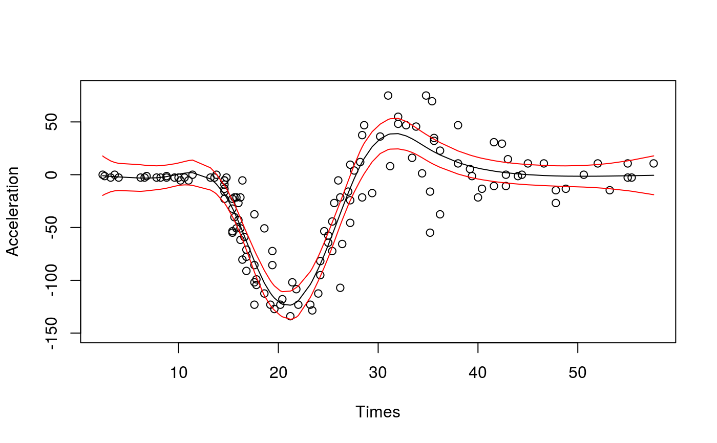
library(qgam); library(MASS)

# Calibrate learning rate on a grid
set.seed(41444)
sigSeq <- seq(1.5, 5, length.out = 10)
closs <- tuneLearn(form = accel~s(times,k=20,bs="ad"),
                   data = mcycle,
                   lsig = sigSeq,
                   qu = 0.5)

plot(sigSeq, closs$loss, type = "b", ylab = "Calibration Loss", xlab = "log(sigma)")

# Pick best log-sigma
best <- sigSeq[ which.min(closs$loss) ]
abline(v = best, lty = 2)

# Fit using the best sigma
fit <- qgam(accel~s(times,k=20,bs="ad"), data = mcycle, qu = 0.5, lsig = best)
summary(fit)
#> 
#> Family: elf 
#> Link function: identity 
#> 
#> Formula:
#> accel ~ s(times, k = 20, bs = "ad")
#> 
#> Parametric coefficients:
#>             Estimate Std. Error z value Pr(>|z|)    
#> (Intercept)   -25.20       1.88   -13.4   <2e-16 ***
#> ---
#> Signif. codes:  0 ‘***’ 0.001 ‘**’ 0.01 ‘*’ 0.05 ‘.’ 0.1 ‘ ’ 1
#> 
#> Approximate significance of smooth terms:
#>           edf Ref.df Chi.sq p-value    
#> s(times) 8.73  10.11  531.3  <2e-16 ***
#> ---
#> Signif. codes:  0 ‘***’ 0.001 ‘**’ 0.01 ‘*’ 0.05 ‘.’ 0.1 ‘ ’ 1
#> 
#> R-sq.(adj) =  0.782   Deviance explained = 71.5%
#> -REML = 608.79  Scale est. = 1         n = 133

pred <- predict(fit, se=TRUE)
plot(mcycle$times, mcycle$accel, xlab = "Times", ylab = "Acceleration",
     ylim = c(-150, 80))
lines(mcycle$times, pred$fit, lwd = 1)
lines(mcycle$times, pred$fit + 2*pred$se.fit, lwd = 1, col = 2)
lines(mcycle$times, pred$fit - 2*pred$se.fit, lwd = 1, col = 2)