Checking residuals conditional density

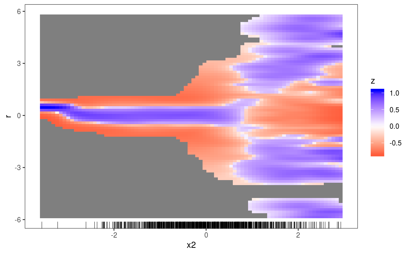
This layer calculates and plots how the empirical conditional density of the residuals, r, differs from its theoretical or model-based counterpart, along a covariate, x.

l_densCheck(n = c(80, 80), bw = NULL, tol = 1e-06, dFun = NULL, ...)

Arguments

n	vector of two positive integers, indicating the number of grid points at which the density is evaluated on the x and r axes.
bw	vector with two positive entries, indicating the bandwidth to be used by the kernel density estimator of p(r|x) along x and r.
tol	small positive numerical tolerance. The estimated density at a certain location is set to NA (hence it will appear white) when it falls below tol/sqrt(2*pi*sig), where sig is the standard deviation of the residuals. Set tol to -1 plot the density on the whole x-y plane, no matter how low it is.
dFun	function used to compute the difference between the empirical (em) and theoretical (th) conditional density of the residuals. By default it is (sqrt(em)-sqrt(th))^(1/3), where th is computed using either a uniform or a normal density, depending on the type of residuals used in the check1D call. It should have as arguments three vectors: .ed (the empirical conditional density), .gr (the points along the y-axis where the density is evaluated) and .y (the residuals).
...	graphical arguments to be passed to ggplot2::geom_raster.

Value

An object of class gamLayer.

Details

This layer is mainly meant to work together with the check1D function. If check1D() is called with residual type == "tunif" or "tnormal", then l_densCheck compares the conditional distribution of the residuals with Unif(0, 1) or N(0, 1). By changing the distance function dFun one could of course change both the distance metric and the reference distribution (see Examples below).

WARNING: if check1D() is called with type != "tunif" or "tnormal", then the default distance used by l_densCheck is
dFun <- function(.ed, .gr, .y) {
d <- dnorm(.gr, 0, sd=sd(.y)) # sd=sd(.y) !!!
d <- sqrt(.ed)-sqrt(d)
return(sign(d)*abs(d)^(1/3))
}
so the residuals are standardized using their own std dev sd(.y). Hence l_densCheck might not detect that the mean estimated variance under the fitted model is different from the residuals variance. Hence it is safer to use residual types "tunif" or "tnormal", or a customized distance function dFun (see below for an example on how to do this).

Examples

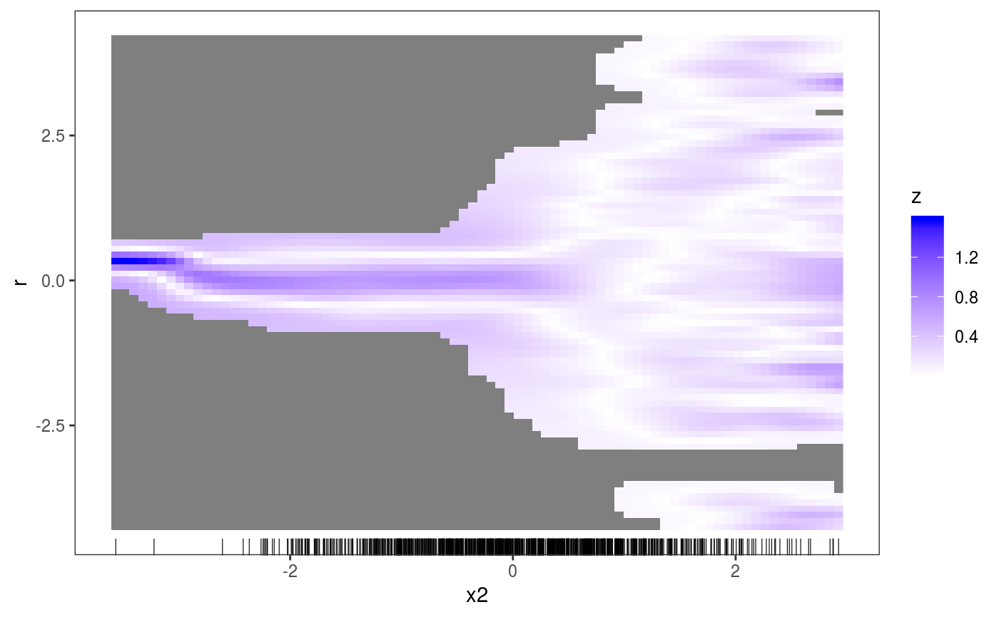
library(mgcViz);
# Dataset where variance increases linearly with x2, for x2 > 0.2
n <- 1e3
x1 <- rnorm(1e3)
x2 <- rnorm(1e3)
dat <- data.frame("x1"=x1,
                  "x2"=x2, "y"=sin(x1) + 0.5*x2^2 + pmax(x2, 0.2)*rnorm(n))
b <- gam(y ~ s(x1)+s(x2), data=dat)
b <- getViz(b)

# (Red) Blue indicates area where the empirical density 
# of the residuals is (lower) higher than it should be under 
# the model (residuals should be N(0, sigma) here).
# Here there are clear signs of heteroscedasticity: 
# the conditional variance is is increasing for x2 > 0.2. 
check1D(b, "x2", type = "tnormal") + l_densCheck() + l_rug()

# Suppose we want to compare the conditional density of the standardized residuals
# not with a Gaussian, but with a Student-t density with 3 degree of freedom.
# We could achieve this as follows:
myDistance <- function(.ed, .gr, .y){
  d <- dt(.gr / sd(.y), df = 3)
  d <- abs( sqrt(.ed) - sqrt(d) ) # We are using absolute difference between sqrt-densities 
}

check1D(b, "x2", type = "response") + l_densCheck(dFun = myDistance) + l_rug()
# NB comparing with a Student density is not useful for this example, but it illustrates
# how both the distance function and the reference density can be customized.