Quantile additive models using qgam and mgcViz
Matteo Fasiolo and Raphael Nedellec
March 04 2020
Source:vignettes/qgam_mgcViz.Rmd
qgam_mgcViz.RmdIntroduction
The qgam R package offers methods for fitting additive quantile regression models based on splines, using the methods described in Fasiolo et al., 2017. It is useful to use qgam together with mgcViz Fasiolo et al., 2018, which extends the basic visualizations provided by mgcv.
The main fitting functions are:
-
qgam()fits an additive quantile regression model to a single quantile. Very similar tomgcv::gam(). It returns an object of classqgam, which inherits frommgcv::gamObject. -
mqgam()fits the same additive quantile regression model to several quantiles. It is more efficient that callingqgam()several times, especially in terms of memory usage. -
qgamV()andmqgamV()are two convenient wrappers that fit quantile GAMs and returngamVizobjects, for whichmgcVizprovides lots of visualizations.
An additive example with four covariates
We simulate some data from the model: \[ y = f_0(x_0)+f_1(x_1)+f_2(x_2)+f_3(x_3)+e,\;\;\; e \sim N(0, 2) \] by doing
library(mgcViz)
set.seed(2)
dat <- gamSim(1, n=1000, dist="normal", scale=2)[c("y", "x0", "x1", "x2", "x3")]
## Gu & Wahba 4 term additive modelWe start by fitting a linear quantile model for the median:
## Estimating learning rate. Each dot corresponds to a loss evaluation.
## qu = 0.5.......done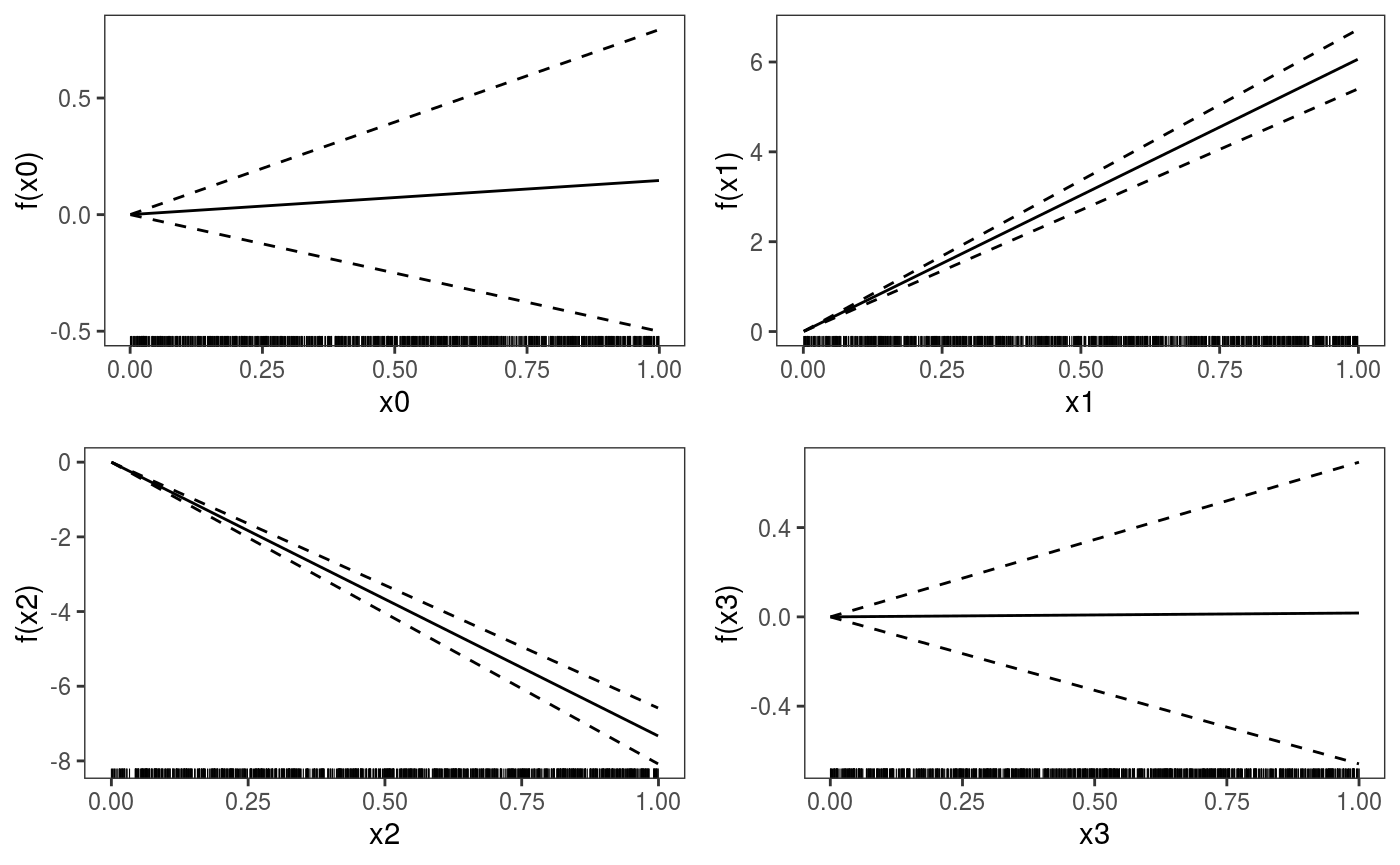 We use
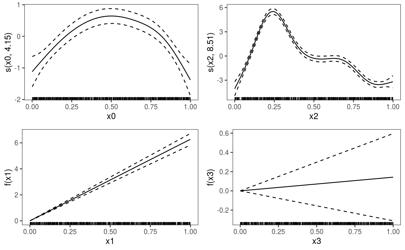
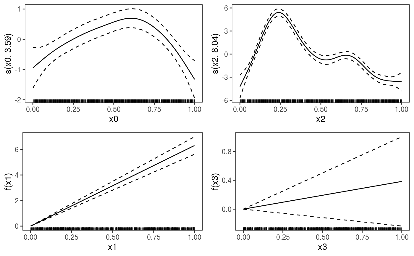
 pages = 1 to plot on a single page, and allTerms to plot also the parametric effects (the plotting method used here plots only smooth or random effects by default).
Should we use a smooth effect of x0? If the effect of x0 was non-linear, we would expect that the number of observations falling below the fit would depart from 0.5, as we move along x0. A rudimental diagnostic plot is:
plot(dat$x0, sign(residuals(fit1)) + rnorm(nrow(dat), 0, 0.05), col = alpha(1, 0.4), pch = 16,
ylab = "Residuals sign", xlab = "x0")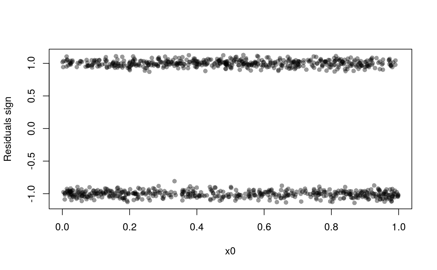 But residual pattern is more visible in the following plot:
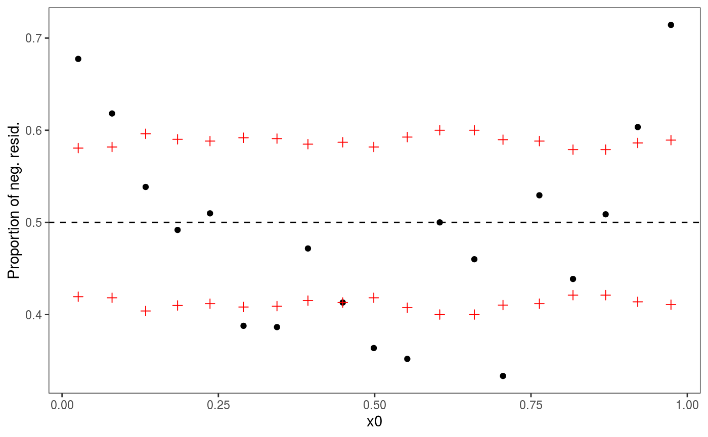 There is definitely a pattern here. An analogous plot along
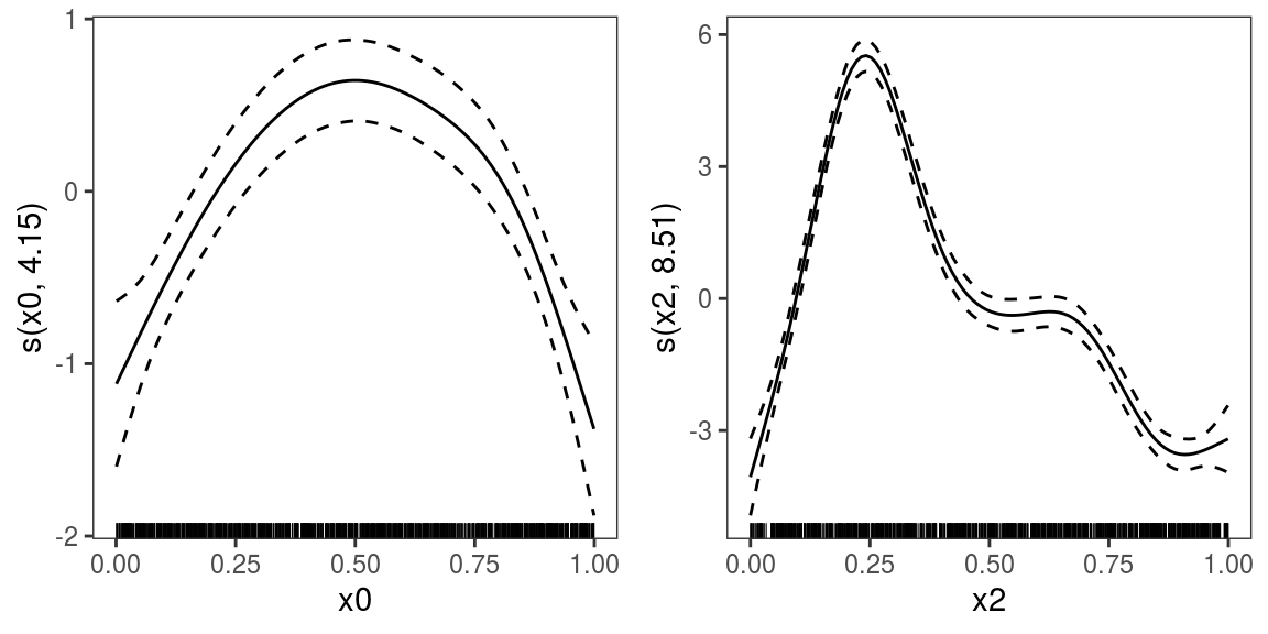
 x2 also shows a residual pattern, hence we consider the model:
## Estimating learning rate. Each dot corresponds to a loss evaluation.
## qu = 0.5.......done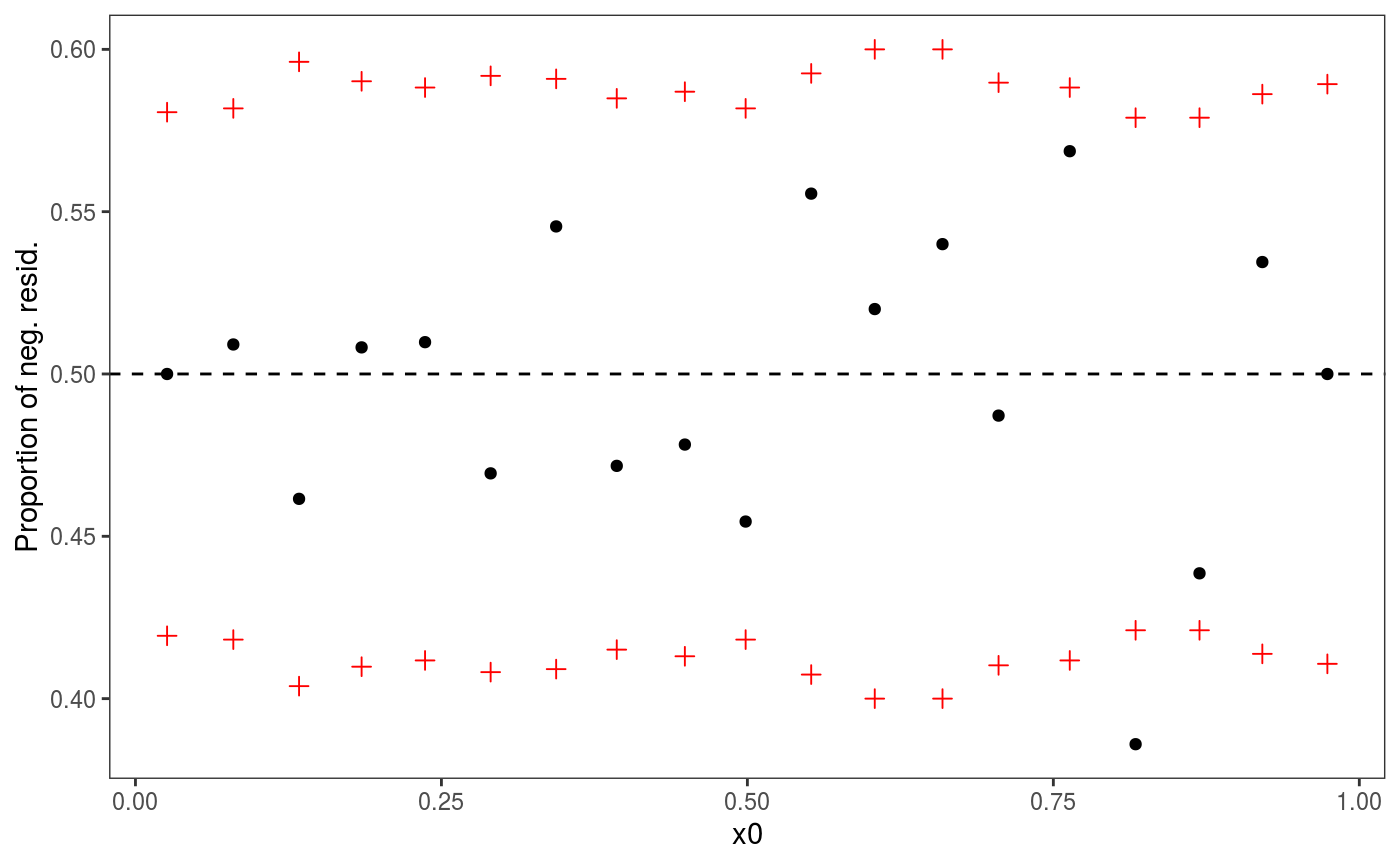 Looks much better, and leads to much lower AIC:
## [1] 764.418We can plot all the smooth effects by doing:
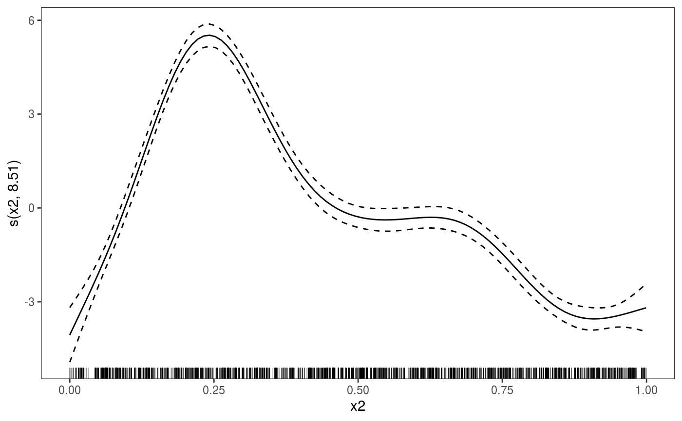
 To print only the second we do
 Now we fit this model to multiple quantiles and plot the fitted effects:
## Estimating learning rate. Each dot corresponds to a loss evaluation.
## qu = 0.5.......done
## qu = 0.3.......done
## qu = 0.7........done
## qu = 0.1........done
## qu = 0.9........done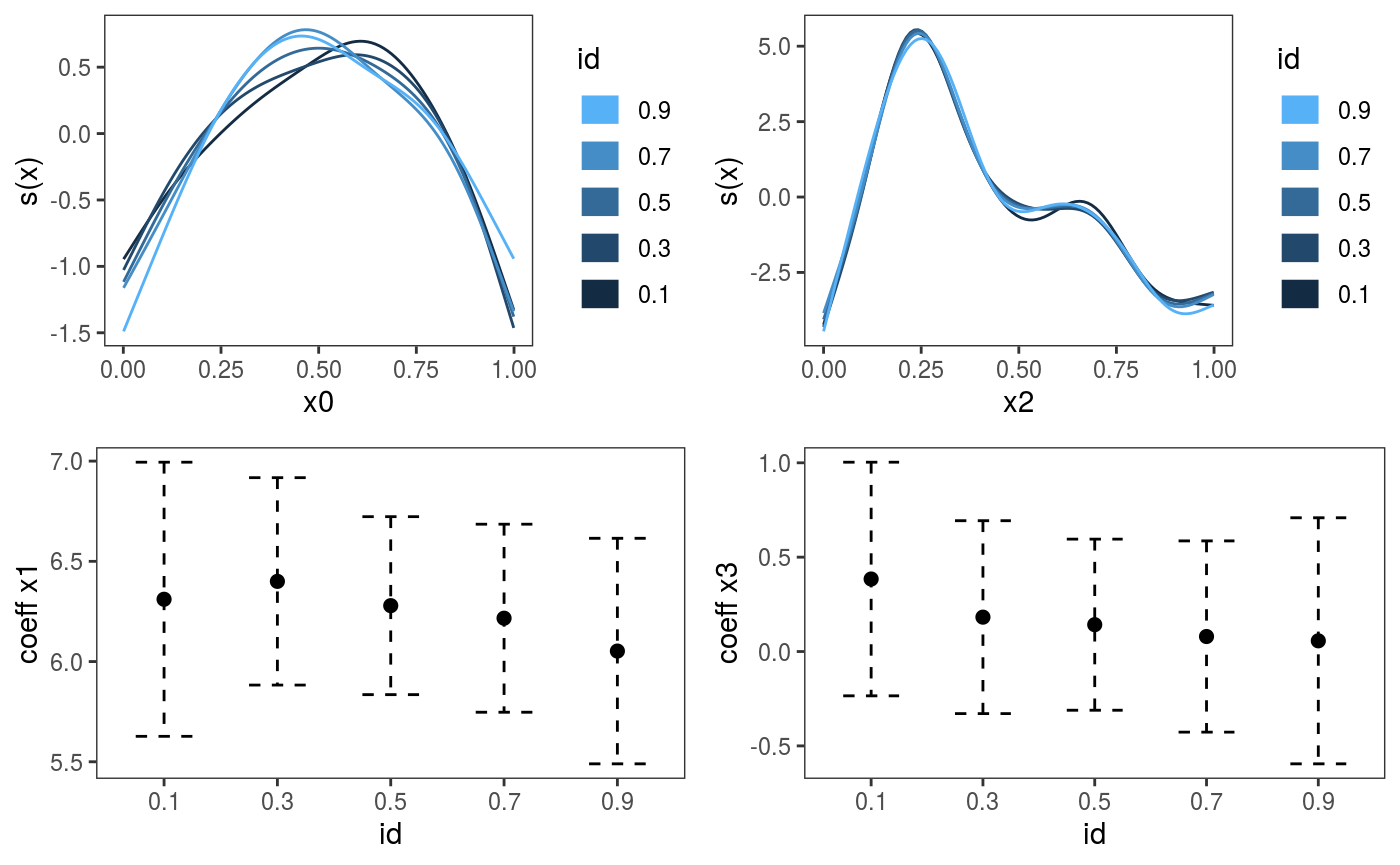
We can manipulate the five fitted quantile GAMs individually, for example
Random effect modelling: lexical decision task
In this experiment participants are presented with a sequence of stimuli and they have to decide, as quickly as possible, whether each stimulus is an existing words (eg. house) or a non-existing word (eg. pensour) by pressing one of two buttons. The variables we consider here are:
-
RTlogarithmically transformed reaction time. -
NativeLanguagea factor with levels English and Other. -
Lengththe word’s length in letters. -
Frequencylogarithmically transformed lemma frequencies as available in the CELEX lexical database. -
Subjectthe id of the individual subjects. -
Trialthe rank of the trial in the experimental list. -
Worda factor with 79 words as levels.
We might be interested in modeling the relation between the response time and length, frequency, native language and trial, and we might want to control for word and subject. We start by loading the data and fitting a simple QGAM model for the median:
library(languageR)
data(lexdec)

lexdec$RT0 <- exp( lexdec$RT ) # Should not need to use log-responses to normalize

fit <- qgamV(RT0 ~ s(Trial) + NativeLanguage + s(Length, k = 5) + s(Frequency),
            data = lexdec, qu = 0.5)
## Estimating learning rate. Each dot corresponds to a loss evaluation.
## qu = 0.5.............done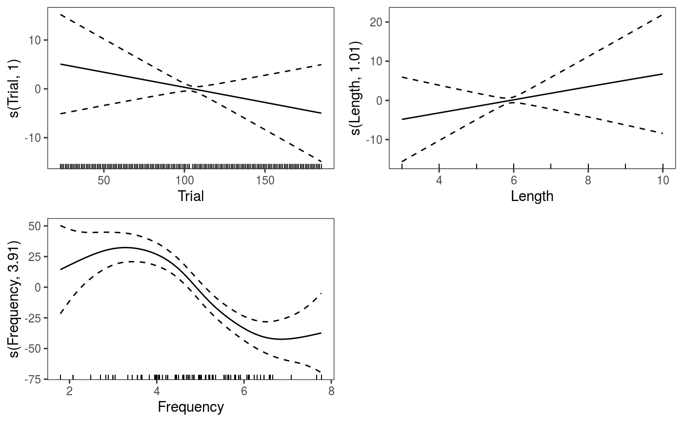 It is natural to ask ourselves whether we should control for
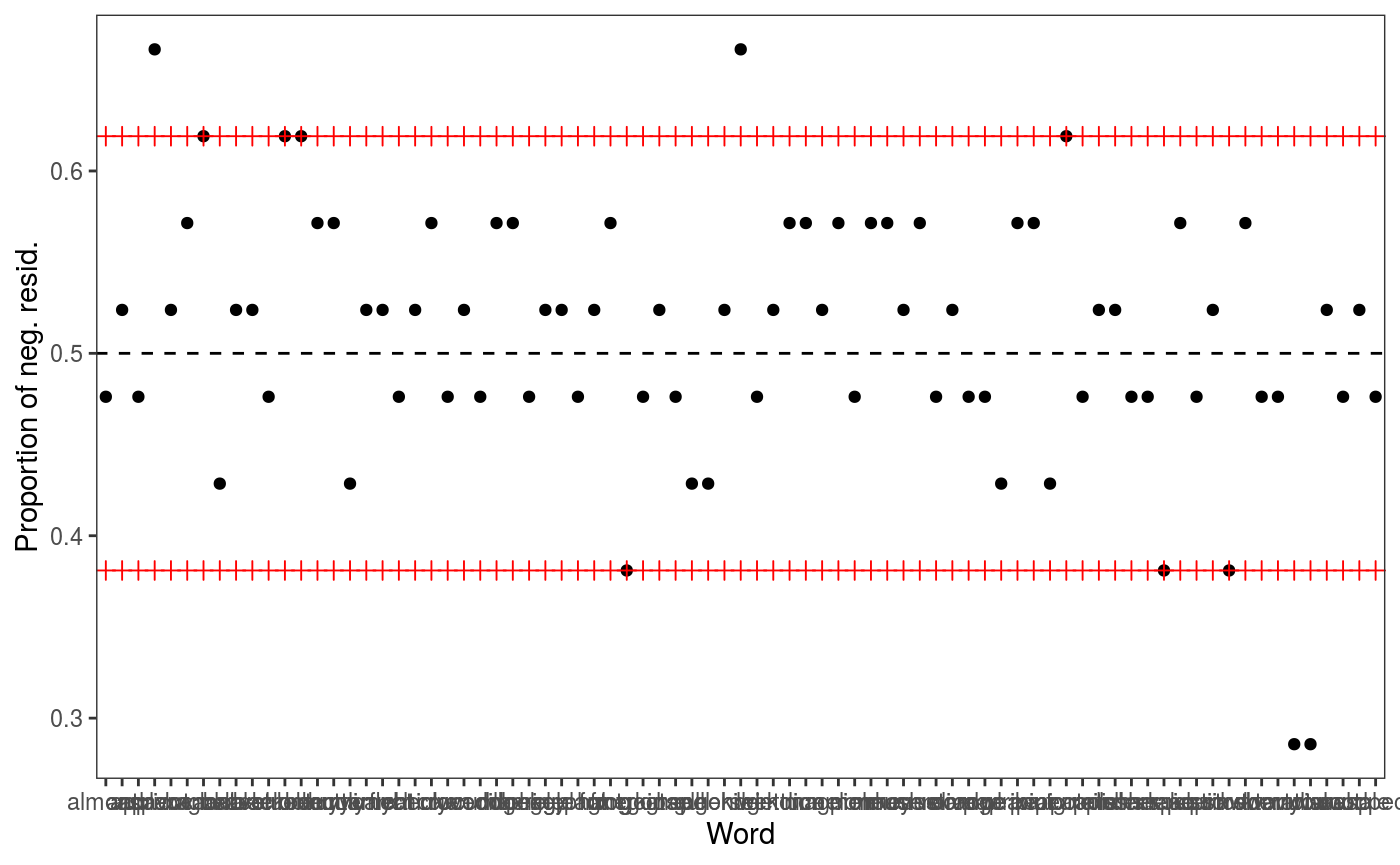
 Subject and for Word:
# check1D(fit, "Subject") would not work because it was not included in the original fit
check1D(fit, lexdec$Subject) + l_gridQCheck1D(qu = 0.5)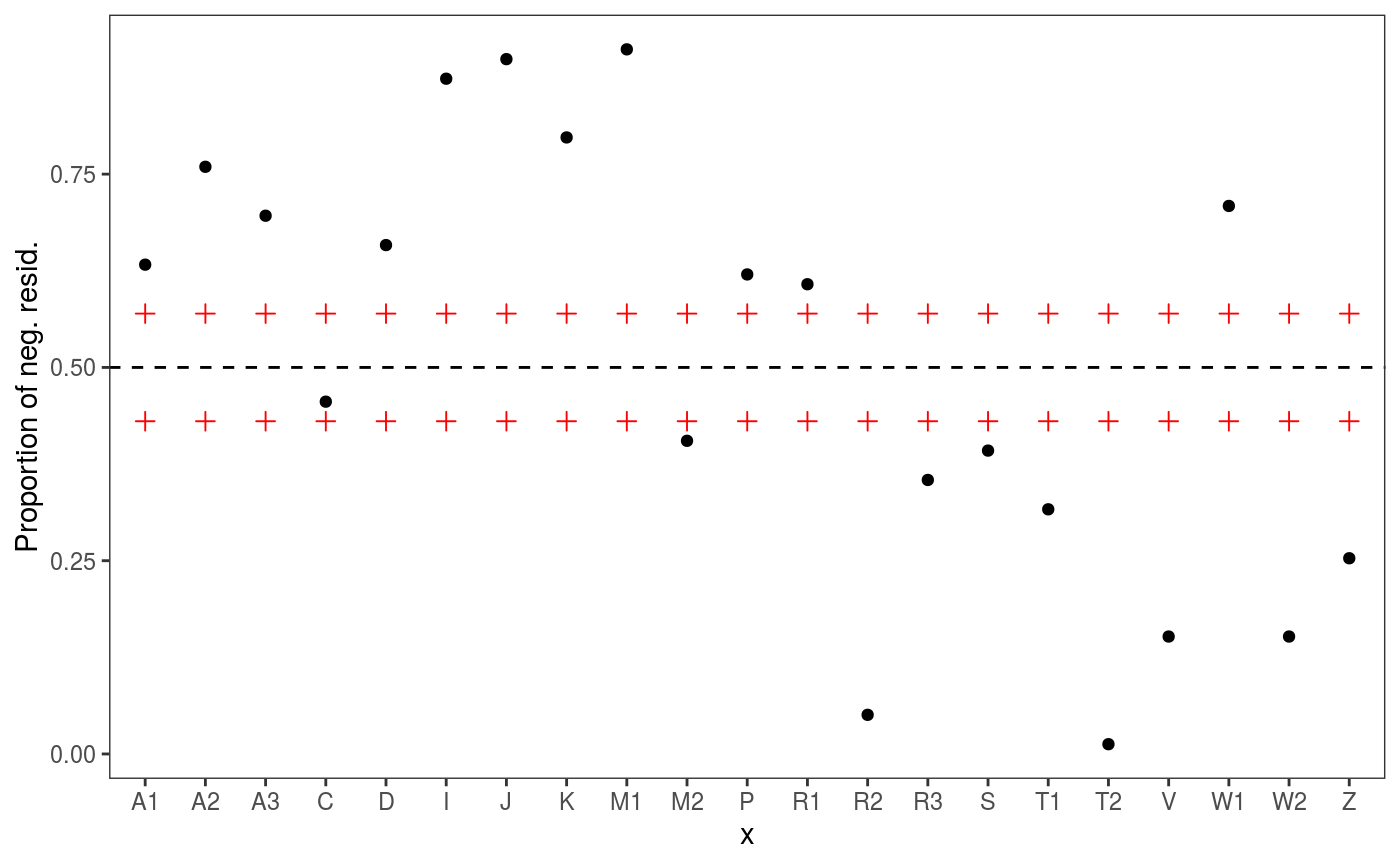
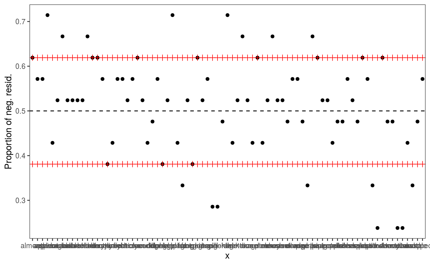 It seems so, hence we refit using two random effects:
fit2 <- qgamV(RT0 ~ s(Trial) + NativeLanguage + s(Length, k = 5) +
                    s(Frequency) + s(Subject, bs = "re") + s(Word, bs = "re"),
            data = lexdec, qu = 0.5)
## Estimating learning rate. Each dot corresponds to a loss evaluation.
## qu = 0.5..........done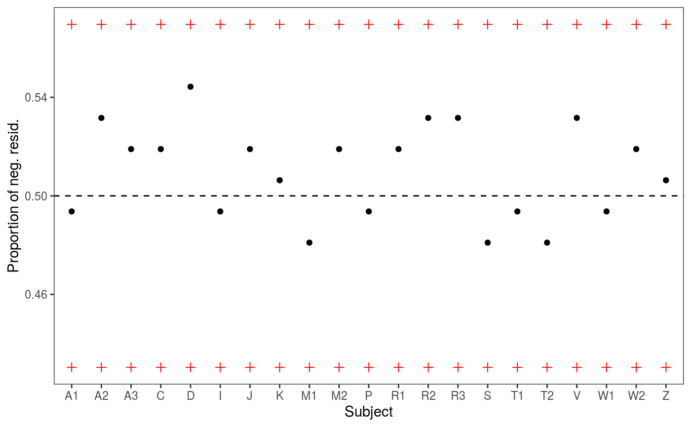
## [1] 817.0046We achieve lower AIC and the residuals checks look better (especially the one for Subject).
A potentially interesting question is then: is the effect of Trial different for native and non-native speakers? We can verify this by using a by-factor smooth:
fit3 <- qgamV(RT0 ~  s(Trial, by = NativeLanguage) + # <- by-factor smooth
                    NativeLanguage + s(Length, k = 5) + s(Frequency) +
                    s(Subject, bs = "re") + s(Word, bs = "re"),
             data = lexdec, qu = 0.5)
## Estimating learning rate. Each dot corresponds to a loss evaluation.
## qu = 0.5...........done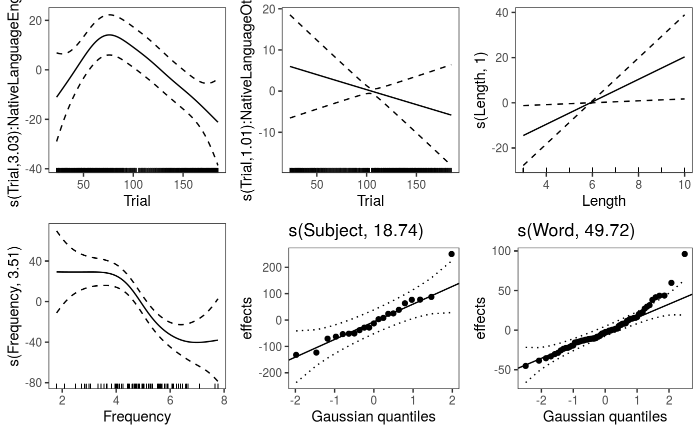 Can look directly at the difference between the by-factor smooths by doing:
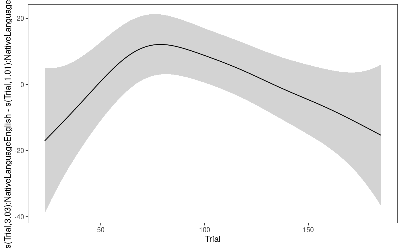 There might be something there, but the difference is not very strong.
Now that we have converged on a (hopefully reasonable) model, we can fit it to several quantiles:
fit5 <- mqgamV(RT0 ~ s(Trial, by = NativeLanguage) + NativeLanguage + s(Length, k = 5) +
                + s(Frequency) + s(Subject, bs = "re") + s(Word, bs = "re"),
                data = lexdec, qu = seq(0.2, 0.8, length.out = 5))
## Estimating learning rate. Each dot corresponds to a loss evaluation.
## qu = 0.5...........done
## qu = 0.35...........done
## qu = 0.65............done
## qu = 0.2..............done
## qu = 0.8...........done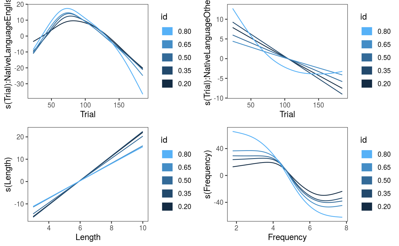
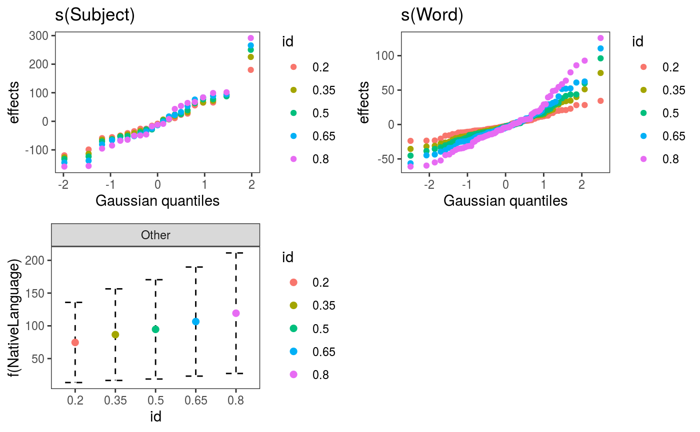 The effects are fairly stable across quantiles, the effect of
 Frequency might be stronger for high quantiles. We can examine the fitted quantile models individually:
##
## Family: elf
## Link function: identity
##
## Formula:
## RT0 ~ s(Trial, by = NativeLanguage) + NativeLanguage + s(Length,
##     k = 5) + +s(Frequency) + s(Subject, bs = "re") + s(Word,
##     bs = "re")
##
## Parametric coefficients:
##                     Estimate Std. Error z value Pr(>|z|)
## (Intercept)           641.78      31.08   20.65   <2e-16 ***
## NativeLanguageOther   119.27      46.95    2.54   0.0111 *
## ---
## Signif. codes:  0 '***' 0.001 '**' 0.01 '*' 0.05 '.' 0.1 ' ' 1
##
## Approximate significance of smooth terms:
##                                   edf Ref.df  Chi.sq  p-value
## s(Trial):NativeLanguageEnglish  2.679  3.320  13.162  0.00732 **
## s(Trial):NativeLanguageOther    1.375  1.653   0.472  0.59694
## s(Length)                       1.007  1.009   1.108  0.29424
## s(Frequency)                    2.793  3.036  35.087 1.37e-07 ***
## s(Subject)                     18.556 19.000 832.680  < 2e-16 ***
## s(Word)                        48.808 76.000 170.439 4.60e-09 ***
## ---
## Signif. codes:  0 '***' 0.001 '**' 0.01 '*' 0.05 '.' 0.1 ' ' 1
##
## R-sq.(adj) =  0.444   Deviance explained = 52.9%
## -REML =  10717  Scale est. = 1         n = 1659
References
Fasiolo, M., Goude, Y., Nedellec, R. and Wood, S. N. (2017). Fast calibrated additive quantile regression. Available at https://arxiv.org/abs/1707.03307
Fasiolo, M., Nedellec, R., Goude, Y. and Wood, S.N. (2018). Scalable visualisation methods for modern Generalized Additive Models. arXiv preprint arXiv:1809.10632.