Checking sign of residuals along one covariate

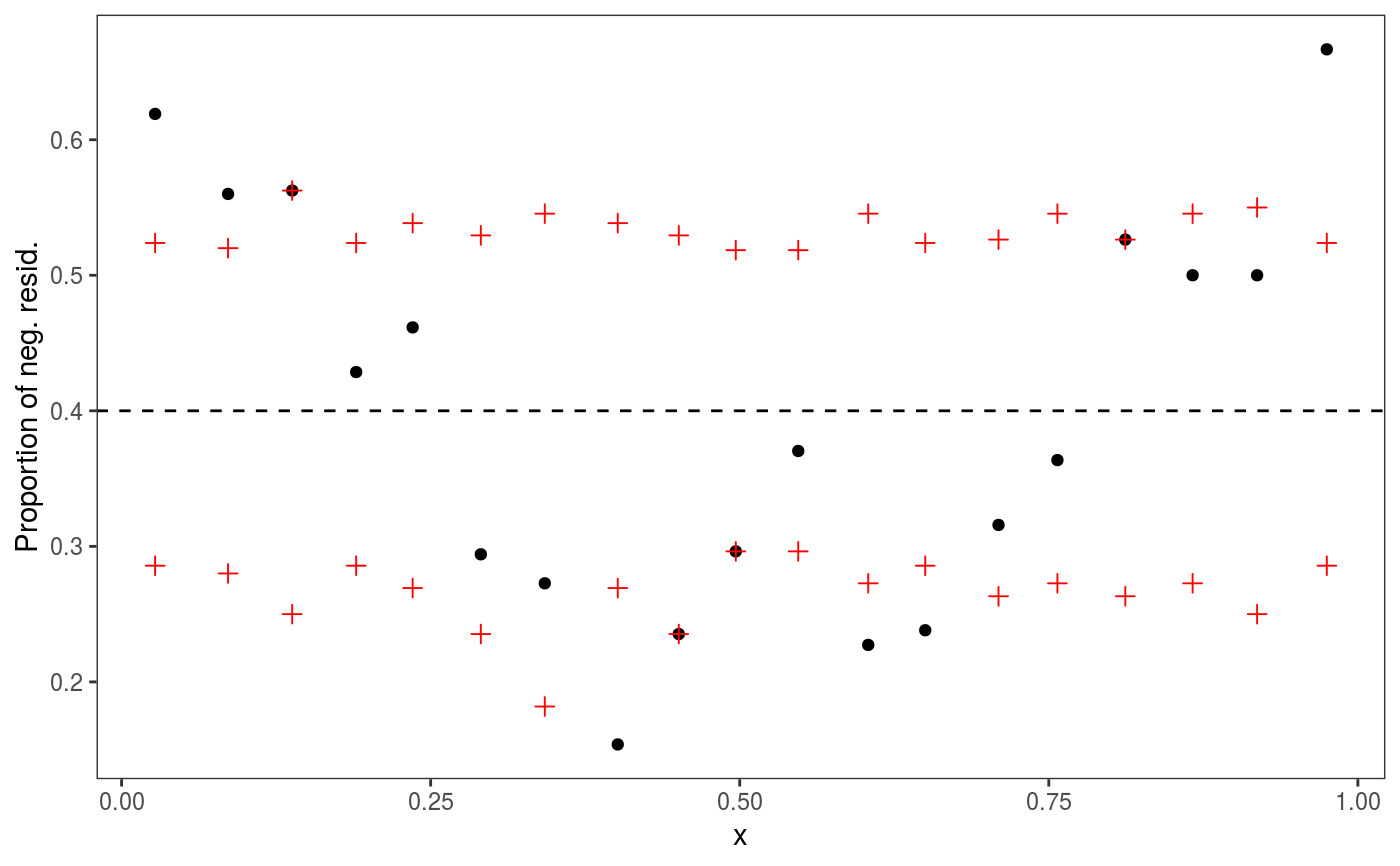
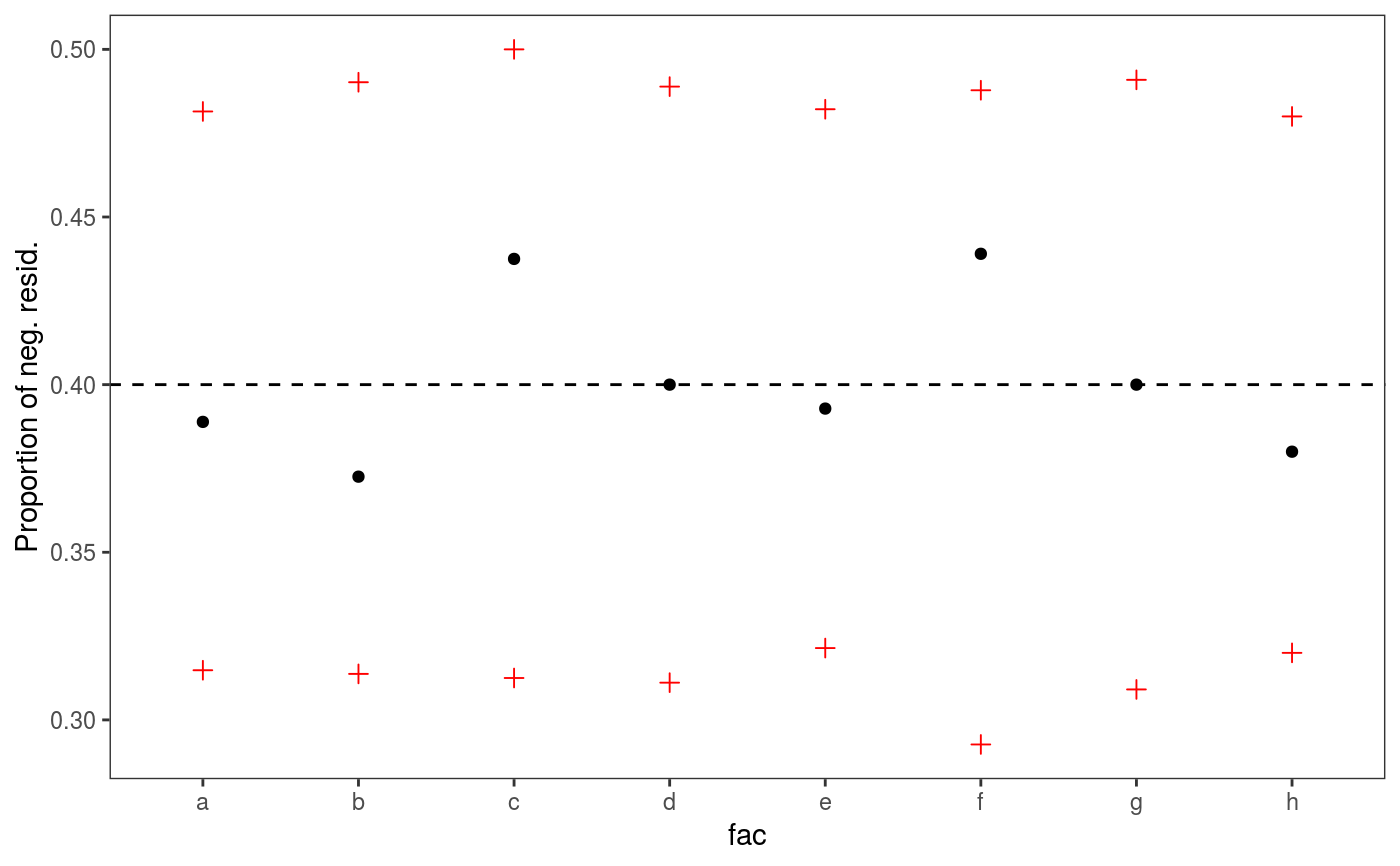
This layer is mainly useful when checking quantile GAMs fitted using the qgam package. The residuals, r, are binned according to the corresponding value of a covariate, x. Then the proportions of negative residuals within each bin are calculated, and compared with the theoretical value, qu. Confidence intervals for the proportion of negative residuals can be derived using binomial quantiles (under an independence assumption). To be used in conjuction with check1D.

l_gridQCheck1D(qu = NULL, n = 20, level = 0.8, ...)

Arguments

qu	the quantile of interest. Should be in (0, 1).
n	number of grid intervals.
level	the level of the confidence intervals plotted.
...	graphical arguments to be passed to ggplot2::geom_point.

Value

An object of class gamLayer

Examples

# Simulate some data
library(mgcViz)
set.seed(3841)
dat <- gamSim(1,n=400,dist="normal",scale=2)
#> Gu & Wahba 4 term additive model
dat$fac <- as.factor( sample(letters[1:8], nrow(dat), replace = TRUE) )
fit <- qgam(y~s(x1)+s(x2)+s(x3)+fac, data=dat, err = 0.05, qu = 0.4)
#> Estimating learning rate. Each dot corresponds to a loss evaluation. 
#> qu = 0.4.................done 
fit <- getViz(fit)

# "x0" effect is missing, but should be there. l_gridQCheck1D shows
# that fraction of negative residuals is quite different from the theoretical 0.4
# in several places along "x0".
check1D(fit, dat$x0) + l_gridQCheck1D(qu = 0.4, n = 20)
# The problem gets better if s(x0) is added to the model.

# Works also with factor variables
check1D(fit, "fac") + l_gridQCheck1D(qu = 0.4)