Binning and checking GAM residuals

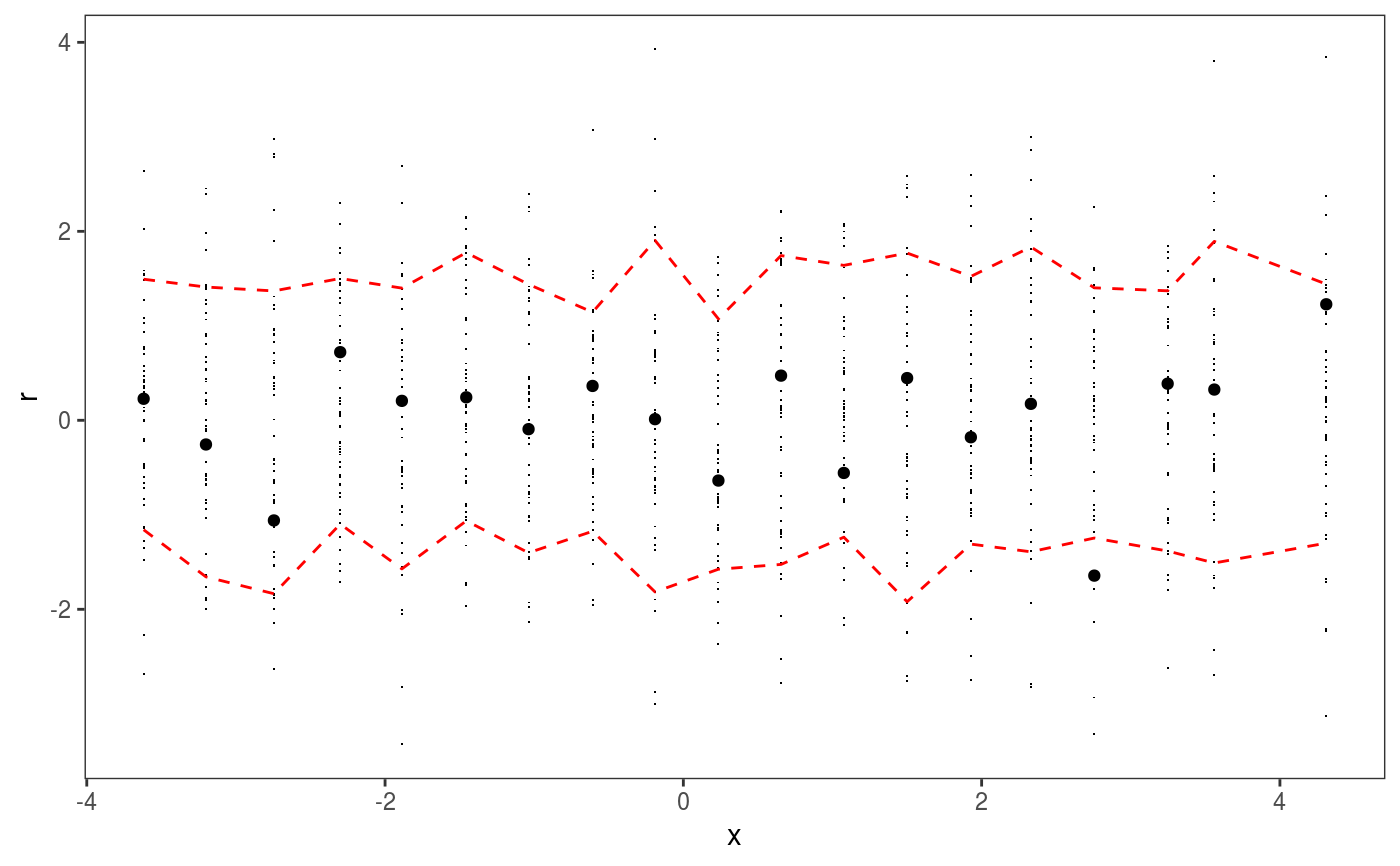
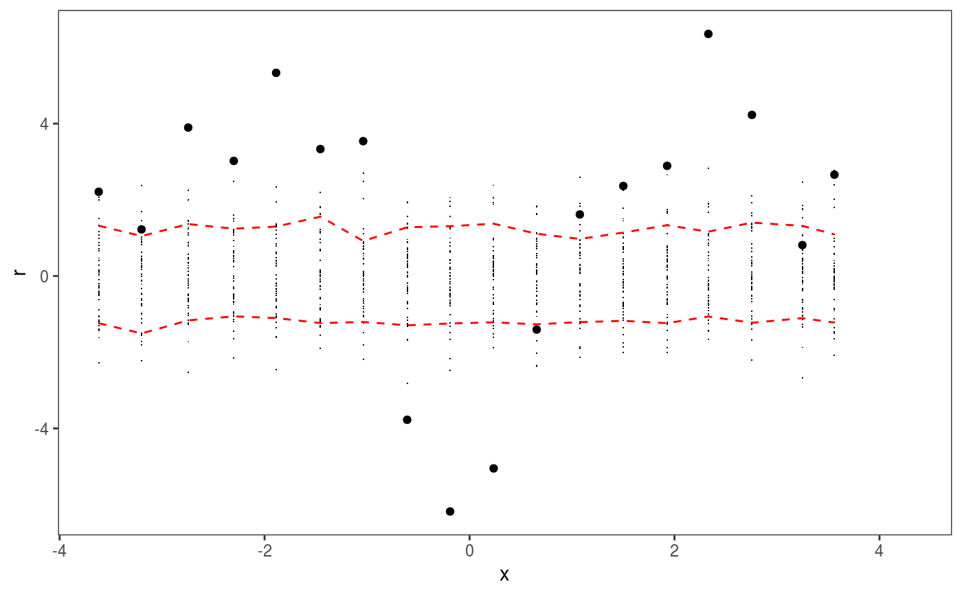
This layer bins the residuals, r, according to the value of the corresponding covariate, x. Then the residuals in each bin are summarized using a scalar-valued statistic. Confidence intervals for the statistic corresponding to each bin can be obtained by simulating residuals from the fitted GAM model, binning and summarizing them. Mainly useful in conjuction with check1D.

l_gridCheck1D(
  gridFun = NULL,
  n = 20,
  level = 0.8,
  stand = "none",
  showReps = TRUE,
  showObs = TRUE,
  ...
)

Arguments

gridFun	scalar-valued function used to summarize the residuals in each bin. It takes a vector as input. By default it is mean(r)*sqrt(length(r)), where r is the vector of residuals in that bin.
n	number of grid intervals along the relevant covariate.
level	the level of the confidence intervals (e.g. 0.9 means 90% intervals).
stand	if "none" the residuals in each bin are transformed by gridFun and the result statistics are plotted directly. If "sc" the statistics in each bin are scaled and centered using the mean and standard deviation of the simulated stats in that bin. If "s" we do only scaling, if "c" only centering.
showReps	if TRUE the individuals simulated statistics are also plotted using small points.
showObs	if TRUE the observed statistics are plotted using large points.
...	graphical arguments to be passed to ggplot2::geom_point.

Value

An object of class gamLayer

Examples

library(mgcViz);
set.seed(4124)
n <- 1e4
x <- rnorm(n); y <- rnorm(n);

# Residuals are heteroscedastic w.r.t. x
ob <- (x)^2 + (y)^2 + (0.2*abs(x) + 1)  * rnorm(n)
b <- bam(ob ~ s(x,k=30) + s(y, k=30), discrete = TRUE)
b <- getViz(b, nsim = 50)

# Don't see much by looking at mean
check1D(b, "x") + l_gridCheck1D()

# Heteroscedasticity clearly visible here
check1D(b, "x") + l_gridCheck1D(gridFun = sd, stand = "sc") # <- we are scaling and centering
# Last point on the right of the rug seems to indicate that a bin is missing.
# It is not an error, only on observation falls in that bin, hence the
# standard deviation is not defined there.