Plot 1D Accumulated Local Effects (ALE)
# S3 method for ALE1D
plot(x, trans = identity, maxpo = 10000, nsim = 0, ...)
Arguments
| x | a 1D ALE effects, produced by the |
|---|---|
| trans | monotonic function to apply to the ALE effect, before plotting. Monotonicity is not checked. |
| maxpo | maximum number of rug lines that will be used by |
| nsim | number of ALE effect curves to be simulated from the posterior distribution. These can be plotted using the l_simLine layer. See Examples section below. |
| ... | currently not used. |
Value
An objects of class plotSmooth.
References
Apley, D.W., and Zhu, J, 2016. Visualizing the effects of predictor variables in black box supervised learning models. arXiv preprint arXiv:1612.08468.
Examples
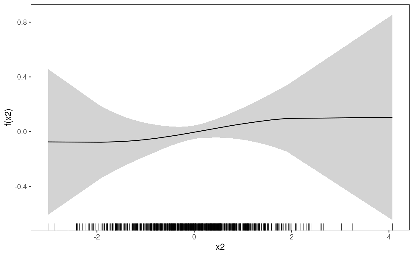
library(mgcViz) # Here x1 and x2 are very correlated, but only # x1 has influence of the response set.seed(4141) n <- 1000 X <- rmvn(n, c(0, 0), matrix(c(1, 0.9, 0.9, 1), 2, 2)) y <- X[ , 1] + 0.2 * X[ , 1]^2 + rnorm(n, 0, 0.8) dat <- data.frame(y = y, x1 = X[ , 1], x2 = X[ , 2]) fit <- gam(y ~ te(x1, x2), data = dat) # Marginal plot suggests that E(y) depends on x2, but # this is due to the correlation between x1 and x2... plot(dat$x2, fit$fitted.values)# ... in fact ALE effect of x2 is flat ... plot(ALE(fit, "x2")) + l_ciPoly() + l_fitLine() + l_rug()# ... while ALE effect of x1 is strong. plot(ALE(fit, "x1", center = 2), nsim = 20) + l_simLine() + l_fitLine()