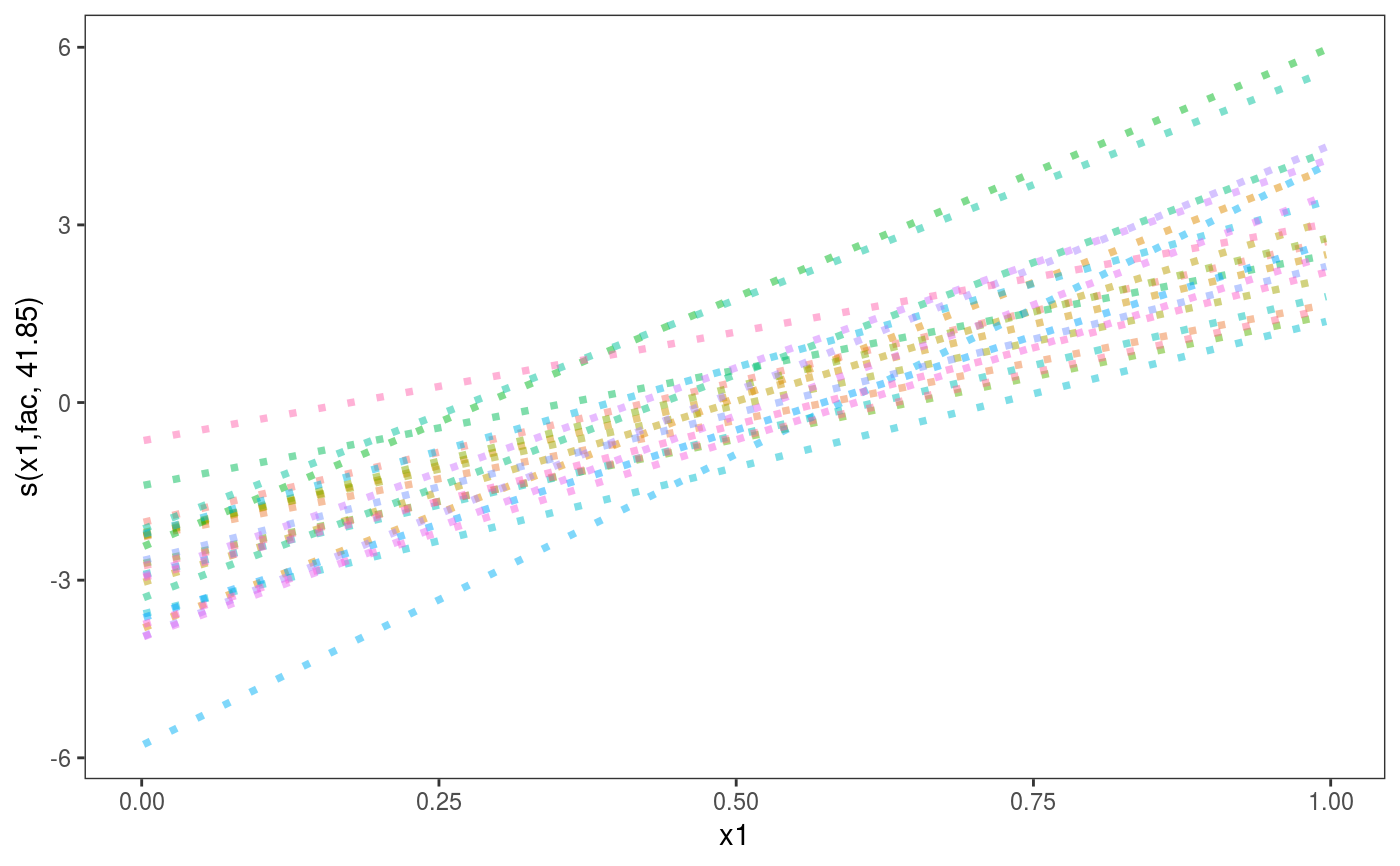
Plotting one dimensional smooth factor interactions

This method should be used to plot smooth effects of class "fs.interaction.1D", that is smooth constructed using the basis bs="tp". See mgcv::s.

# S3 method for fs.interaction.1D
plot(x, n = 100, xlim = NULL, trans = identity, ...)

Arguments

x	a smooth effect object.
n	number of grid points used to compute main effect and c.i. lines. For a nice smooth plot this needs to be several times the estimated degrees of freedom for the smooth.
xlim	if supplied then this pair of numbers are used as the x limits for the plot.
trans	monotonic function to apply to the smooth and residuals, before plotting. Monotonicity is not checked.
...	currently unused.

Value

An object of class c("plotSmooth", "gg").

Examples

library(mgcViz)
set.seed(0)
## simulate data...
f0 <- function(x) 2 * sin(pi * x)
f1 <- function(x, a = 2, b = -1) exp(a * x) + b
f2 <- function(x) 0.2 * x^11 * (10 * (1 - x))^6 + 10 *
  (10 * x)^3 * (1 - x)^10
n <- 500; nf <- 25
fac <- sample(1:nf, n, replace = TRUE)
x0 <- runif(n); x1 <- runif(n); x2 <- runif(n)
a <- rnorm(nf) * .2 + 2; b <- rnorm(nf) * .5
f <- f0(x0) + f1(x1, a[fac], b[fac]) + f2(x2)
fac <- factor(fac)
y <- f + rnorm(n) * 2
## so response depends on global smooths of x0 and
## x2, and a smooth of x1 for each level of fac.

## fit model (note p-values not available when fit
## using gamm)...
bm <- gamm(y ~ s(x0)+ s(x1, fac, bs = "fs", k = 5) + s(x2, k = 20))
v <- getViz(bm$gam)

# Plot with fitted effects and changing title 
plot(sm(v, 2)) + l_fitLine(alpha = 0.6) + labs(title = "Smooth factor interactions")

# Changing plotting limits
plot(sm(v, 2)) + l_fitLine() + ylim(-0.5, 0.5) + xlim(0.25, 0.75)

# Change line type and remove legend
plot(sm(v, 2)) + l_fitLine(size = 1.3, linetype="dotted") +
                 theme(legend.position="none")

# Clustering smooth effects in 3 groups
plot(sm(v, 2)) + l_fitLine(colour = "grey") +
                 l_clusterLine(centers = 3, a.clu = list(nstart = 100))