Plotting one dimensional smooth effects
Source:R/plot_mgcv_smooth_1D.R, R/plot_multi_mgcv_smooth_1D.R
plot.mgcv.smooth.1D.RdPlotting method for one dimensional smooth effects.
# S3 method for mgcv.smooth.1D
plot(
  x,
  n = 100,
  xlim = NULL,
  maxpo = 10000,
  trans = identity,
  unconditional = FALSE,
  seWithMean = FALSE,
  nsim = 0,
  ...
)

# S3 method for multi.mgcv.smooth.1D
plot(
  x,
  n = 100,
  xlim = NULL,
  maxpo = 10000,
  trans = identity,
  unconditional = FALSE,
  seWithMean = FALSE,
  asFact = NULL,
  ...
)
Arguments
| x | a smooth effect object, extracted using mgcViz::sm. |
|---|---|
| n | number of grid points used to compute main effect and c.i. lines. For a nice smooth plot this needs to be several times the estimated degrees of freedom for the smooth. |
| xlim | if supplied then this pair of numbers are used as the x limits for the plot. |
| maxpo | maximum number of residuals points that will be used by layers such as
|
| trans | monotonic function to apply to the smooth and residuals, before plotting. Monotonicity is not checked. |
| unconditional | if |
| seWithMean | if TRUE the component smooths are shown with confidence intervals that include the uncertainty about the overall mean. If FALSE then the uncertainty relates purely to the centred smooth itself. Marra and Wood (2012) suggests that TRUE results in better coverage performance, and this is also suggested by simulation. |
| nsim | number of smooth effect curves to be simulated from the posterior distribution. These can be plotted using the l_simLine layer. See Examples section below. |
| ... | currently unused. |
| asFact | determines whether to use a factor or colour bar legend for plot.multi.mgcv.smooth.1D.
When working with models fitted with mqgamV, the default is
|
Value
An objects of class plotSmooth.
References
Marra, G and S.N. Wood (2012) Coverage Properties of Confidence Intervals for Generalized Additive Model Components. Scandinavian Journal of Statistics.
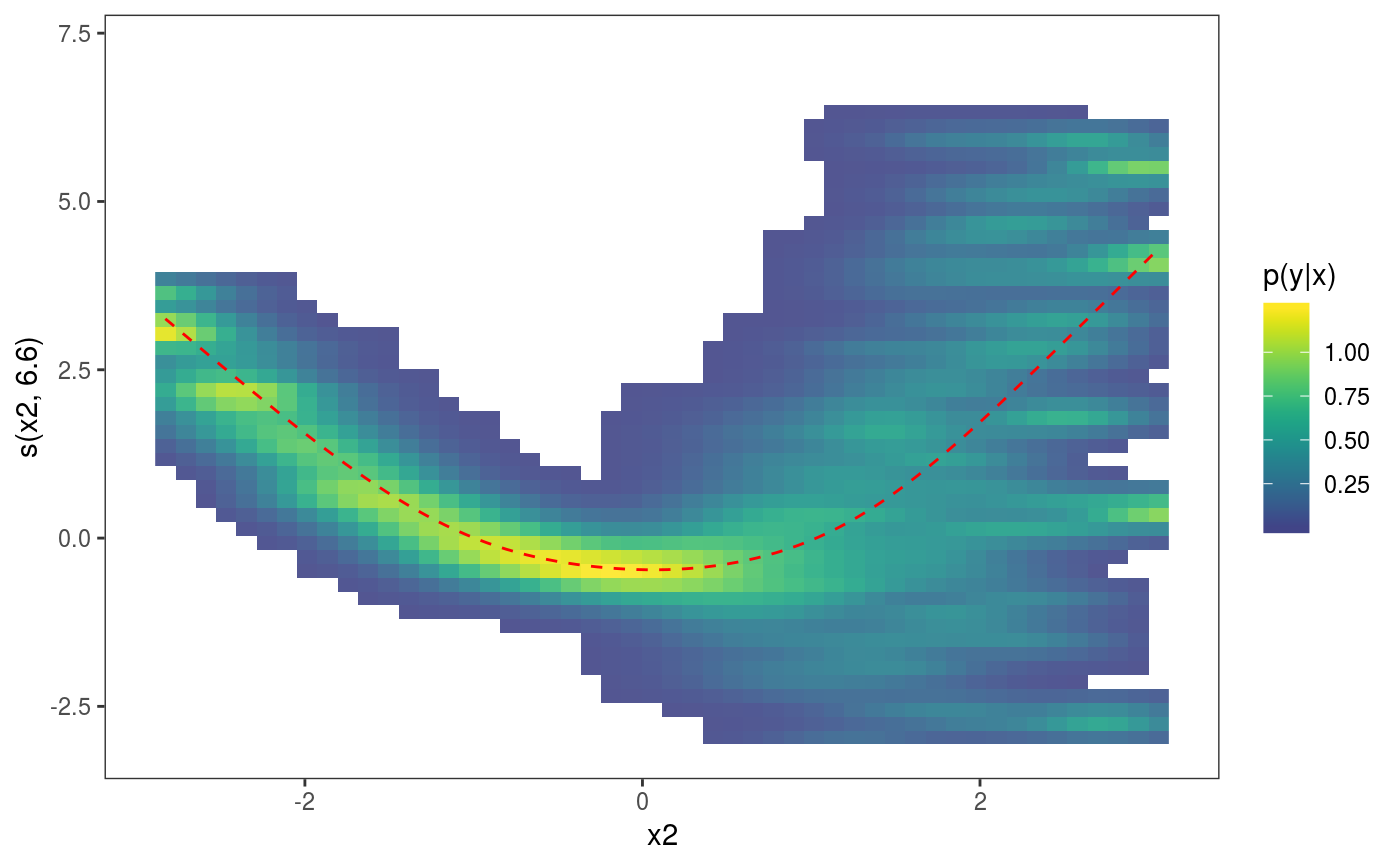
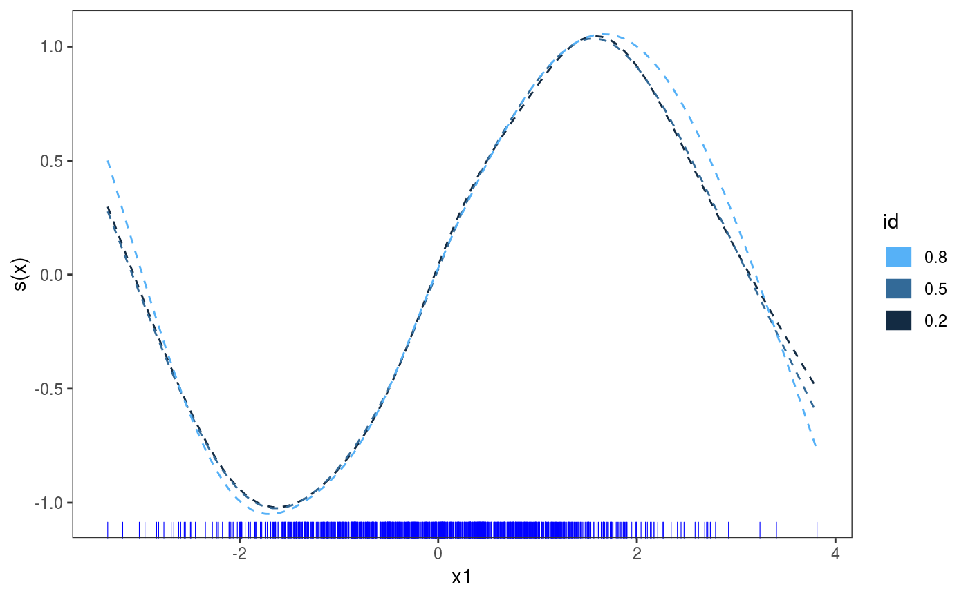
Examples
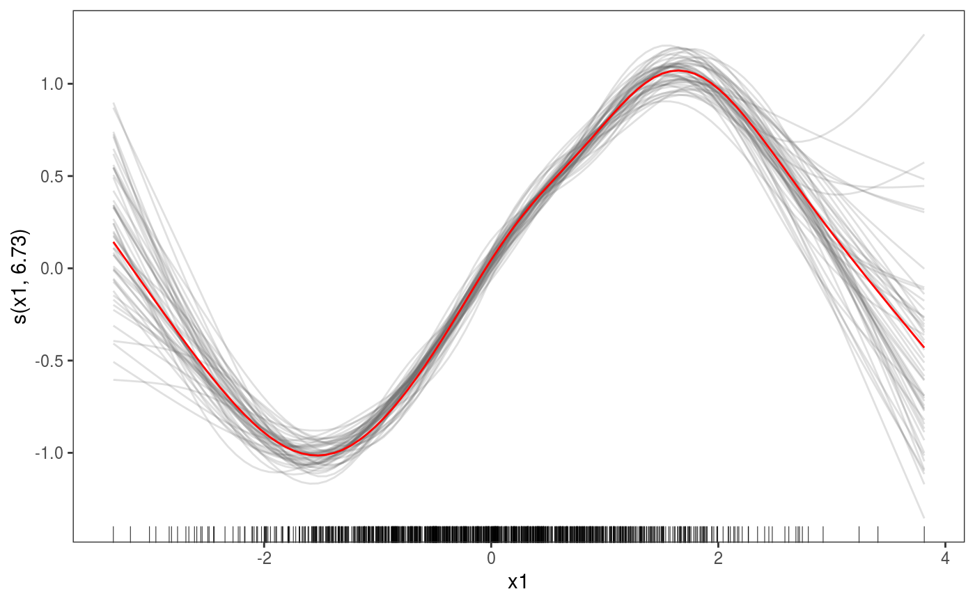
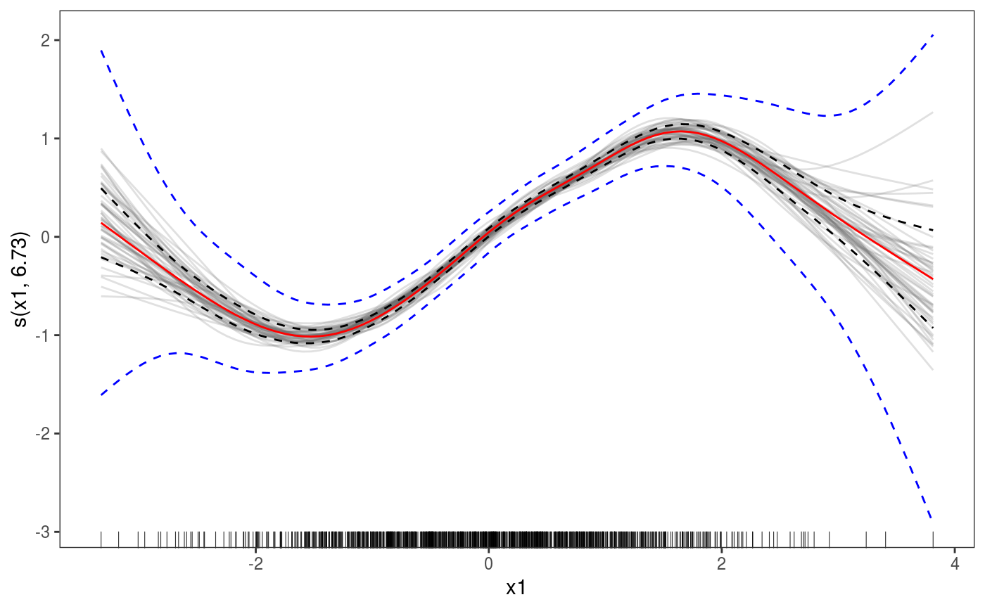
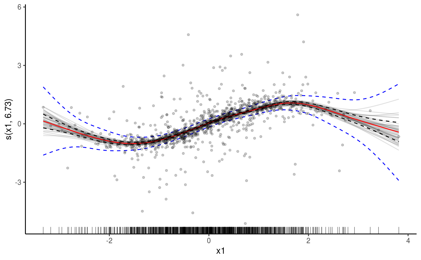
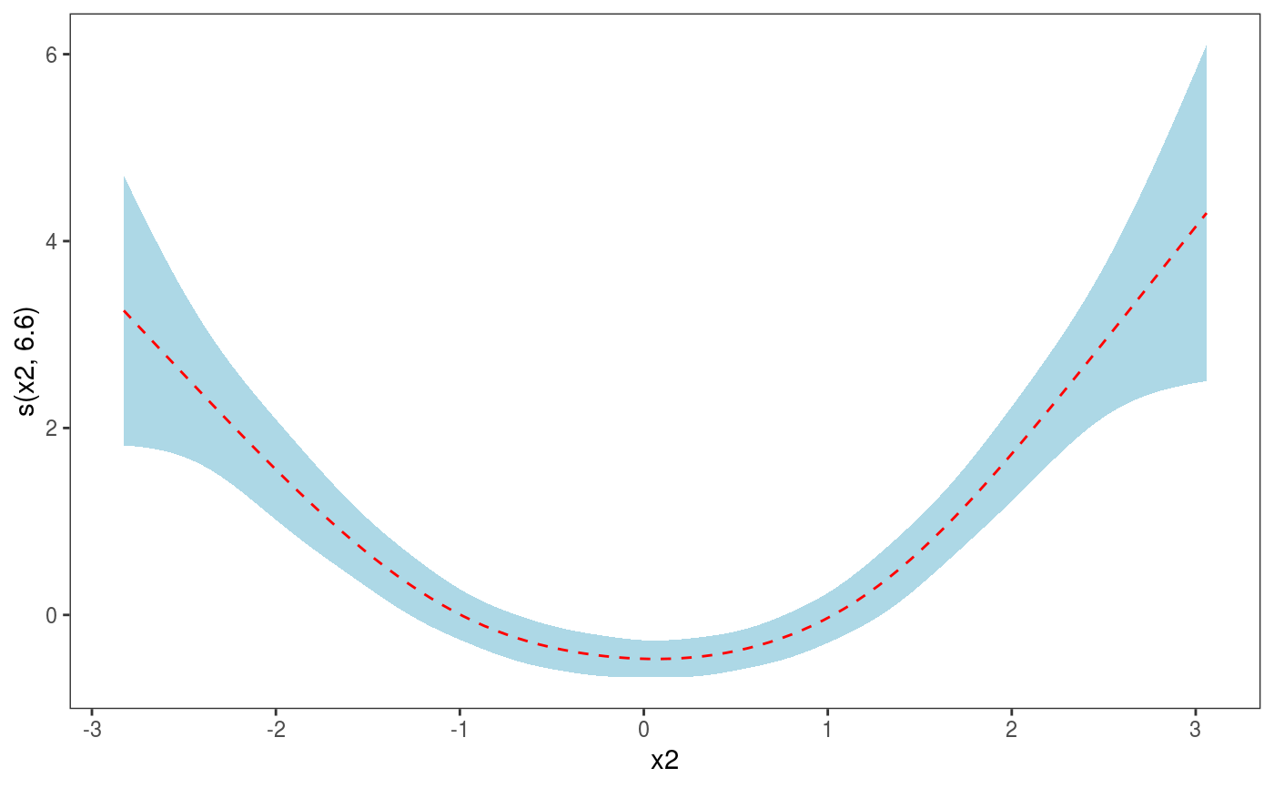
library(mgcViz) n <- 1e3 x1 <- rnorm(n) x2 <- rnorm(n) dat <- data.frame("x1" = x1, "x2" = x2, "y" = sin(x1) + 0.5 * x2^2 + pmax(x2, 0.2) * rnorm(n)) b <- bamV(y ~ s(x1)+s(x2), data = dat, method = "fREML", aGam = list(discrete = TRUE)) o <- plot(sm(b, 1), nsim = 50) # 50 posterior simulations # Plot with fitted effect + posterior simulations + rug on x axis ( o <- o + l_simLine() + l_fitLine(colour = "red") + l_rug(alpha = 0.8) )# Add CI lines at 1*sigma and 5*sigma ( o <- o + l_ciLine(mul = 1) + l_ciLine(mul = 5, colour = "blue", linetype = 2) )# Add partial residuals and change theme ( o + l_points(shape = 19, size = 1, alpha = 0.2) + theme_classic() )# Get second effect plot o2 <- plot( sm(b, 2) ) # Plot it with polygon for partial residuals o2 + l_ciPoly(mul = 5, fill = "light blue") + l_fitLine(linetype = 2, colour = "red")# Plot is with conditional density of partial residuals o2 + l_dens(type = "cond", alpha = 0.9) + l_fitLine(linetype = 2, colour = "red")######## # Quantile GAM example ######## # Fit model b <- mqgamV(y ~ s(x1) + s(x2), qu = c(0.2, 0.5, 0.8), data = dat)#> Estimating learning rate. Each dot corresponds to a loss evaluation. #> qu = 0.5..........done #> qu = 0.2...............done #> qu = 0.8.............#>#> ...#>#> .#>#> .done