Plotting two dimensional smooth effects
Source:R/plot_mgcv_smooth_2D.R, R/plot_multi_mgcv_smooth_2D.R
plot.mgcv.smooth.2D.RdPlotting method for two dimensional smooth effects.
# S3 method for mgcv.smooth.2D
plot(
  x,
  n = 40,
  xlim = NULL,
  ylim = NULL,
  maxpo = 10000,
  too.far = 0.1,
  trans = identity,
  seWithMean = FALSE,
  unconditional = FALSE,
  ...
)

# S3 method for multi.mgcv.smooth.2D
plot(
  x,
  n = 30,
  xlim = NULL,
  ylim = NULL,
  maxpo = 10000,
  too.far = 0.1,
  trans = identity,
  seWithMean = FALSE,
  unconditional = FALSE,
  a.facet = list(),
  ...
)
Arguments
| x | a smooth effect object, extracted using mgcViz::sm. |
|---|---|
| n | sqrt of the number of grid points used to compute the effect plot. |
| xlim | if supplied then this pair of numbers are used as the x limits for the plot. |
| ylim | if supplied then this pair of numbers are used as the y limits for the plot. |
| maxpo | maximum number of residuals points that will be used by layers such as
|
| too.far | if greater than 0 then this is used to determine when a location is too far from data to be plotted. This is useful since smooths tend to go wild away from data. The data are scaled into the unit square before deciding what to exclude, and too.far is a distance within the unit square. Setting to zero can make plotting faster for large datasets, but care then needed with interpretation of plots. |
| trans | monotonic function to apply to the smooth and residuals, before plotting. Monotonicity is not checked. |
| seWithMean | if TRUE the component smooths are shown with confidence intervals that include the uncertainty about the overall mean. If FALSE then the uncertainty relates purely to the centred smooth itself. Marra and Wood (2012) suggests that TRUE results in better coverage performance, and this is also suggested by simulation. |
| unconditional | if |
| ... | currently unused. |
| a.facet | arguments to be passed to ggplot2::facet_wrap or ggplot2::facet_grid. The former gets
called when |
Value
An objects of class plotSmooth.
References
Marra, G and S.N. Wood (2012) Coverage Properties of Confidence Intervals for Generalized Additive Model Components. Scandinavian Journal of Statistics.
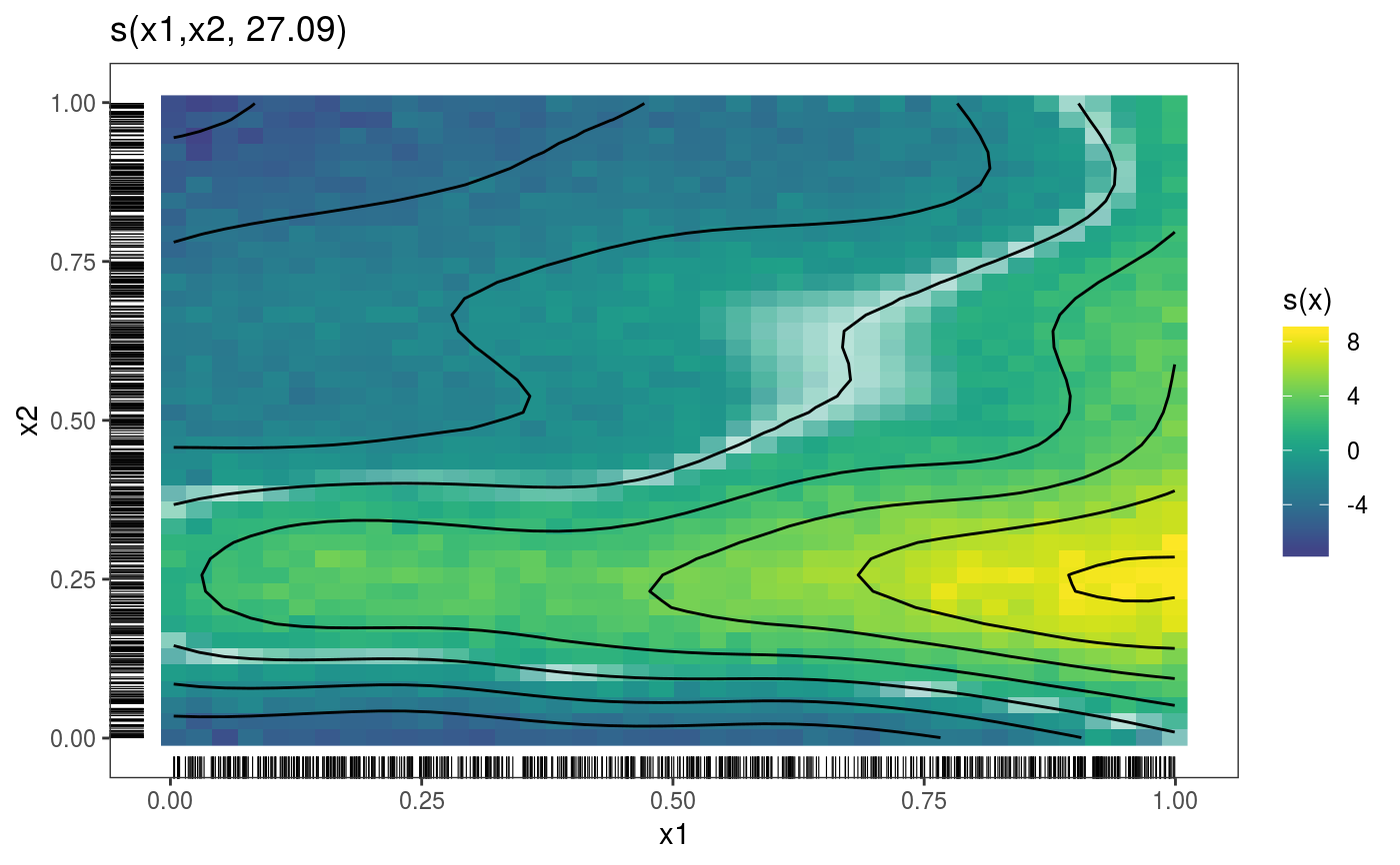
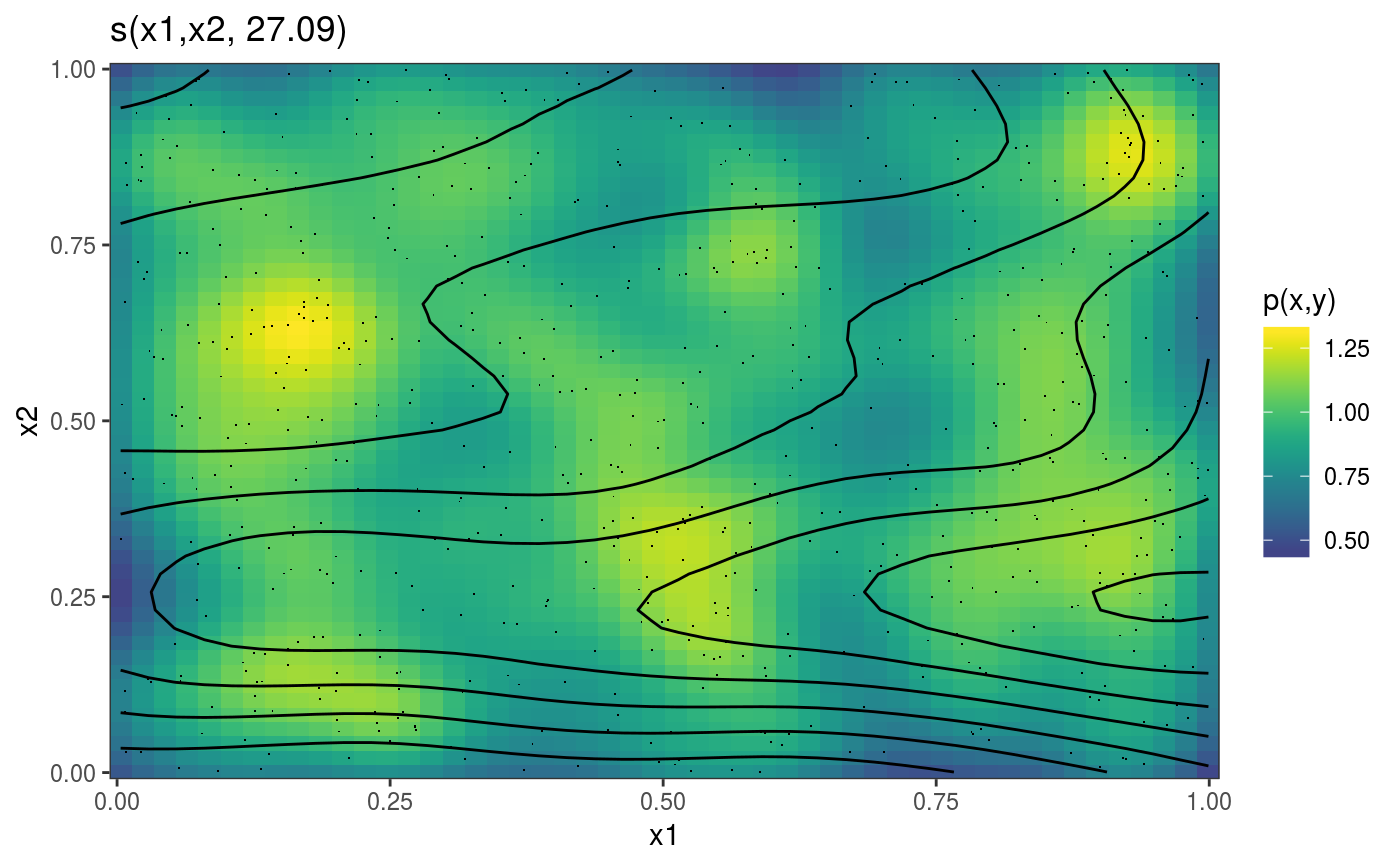
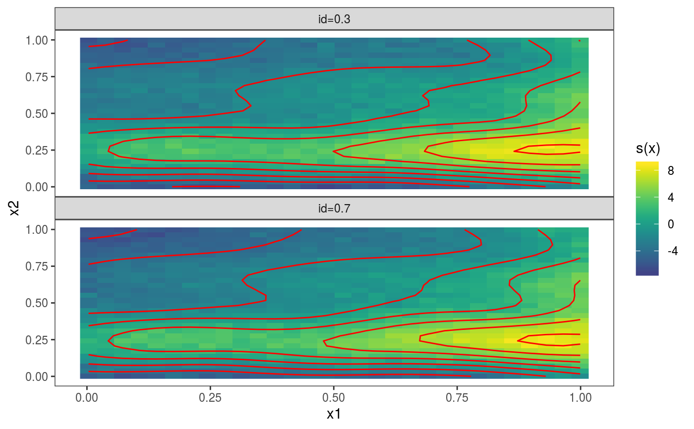
Examples
library(mgcViz) set.seed(2) ## simulate some data... dat <- gamSim(1, n = 700, dist = "normal", scale = 2)#> Gu & Wahba 4 term additive modelb <- gam(y ~ s(x0) + s(x1, x2) + s(x3), data = dat, method = "REML") b <- getViz(b) # Plot 2D effect with noised-up raster, contour and rug for design points # Opacity is proportional to the significance of the effect plot(sm(b, 2)) + l_fitRaster(pTrans = zto1(0.05, 2, 0.1), noiseup = TRUE) + l_rug() + l_fitContour()# Plot contour of effect joint density of design points plot(sm(b, 2)) + l_dens(type = "joint") + l_points() + l_fitContour() + coord_cartesian(expand = FALSE) # Fill the plot### # Quantile GAM example ### b <- mqgamV(y ~ s(x0) + s(x1, x2) + s(x3), qu = c(0.3, 0.7), data = dat)#> Estimating learning rate. Each dot corresponds to a loss evaluation. #> qu = 0.7........done #> qu = 0.3.........done