Plotting Markov random field smooths

This is the plotting method for Markov random field smooths.

# S3 method for mrf.smooth
plot(x, trans = identity, seWithMean = FALSE, unconditional = FALSE, ...)

Arguments

x	a smooth effect object, extracted using mgcViz::sm.
trans	monotonic function to apply to the smooth and residuals, before plotting. Monotonicity is not checked.
seWithMean	if TRUE the component smooths are shown with confidence intervals that include the uncertainty about the overall mean. If FALSE then the uncertainty relates purely to the centred smooth itself. Marra and Wood (2012) suggests that TRUE results in better coverage performance, and this is also suggested by simulation.
unconditional	if TRUE then the smoothing parameter uncertainty corrected covariance matrix is used to compute uncertainty bands, if available. Otherwise the bands treat the smoothing parameters as fixed.
...	currently unused.

Value

An objects of class plotSmooth.

References

Marra, G and S.N. Wood (2012) Coverage Properties of Confidence Intervals for Generalized Additive Model Components. Scandinavian Journal of Statistics.

Examples

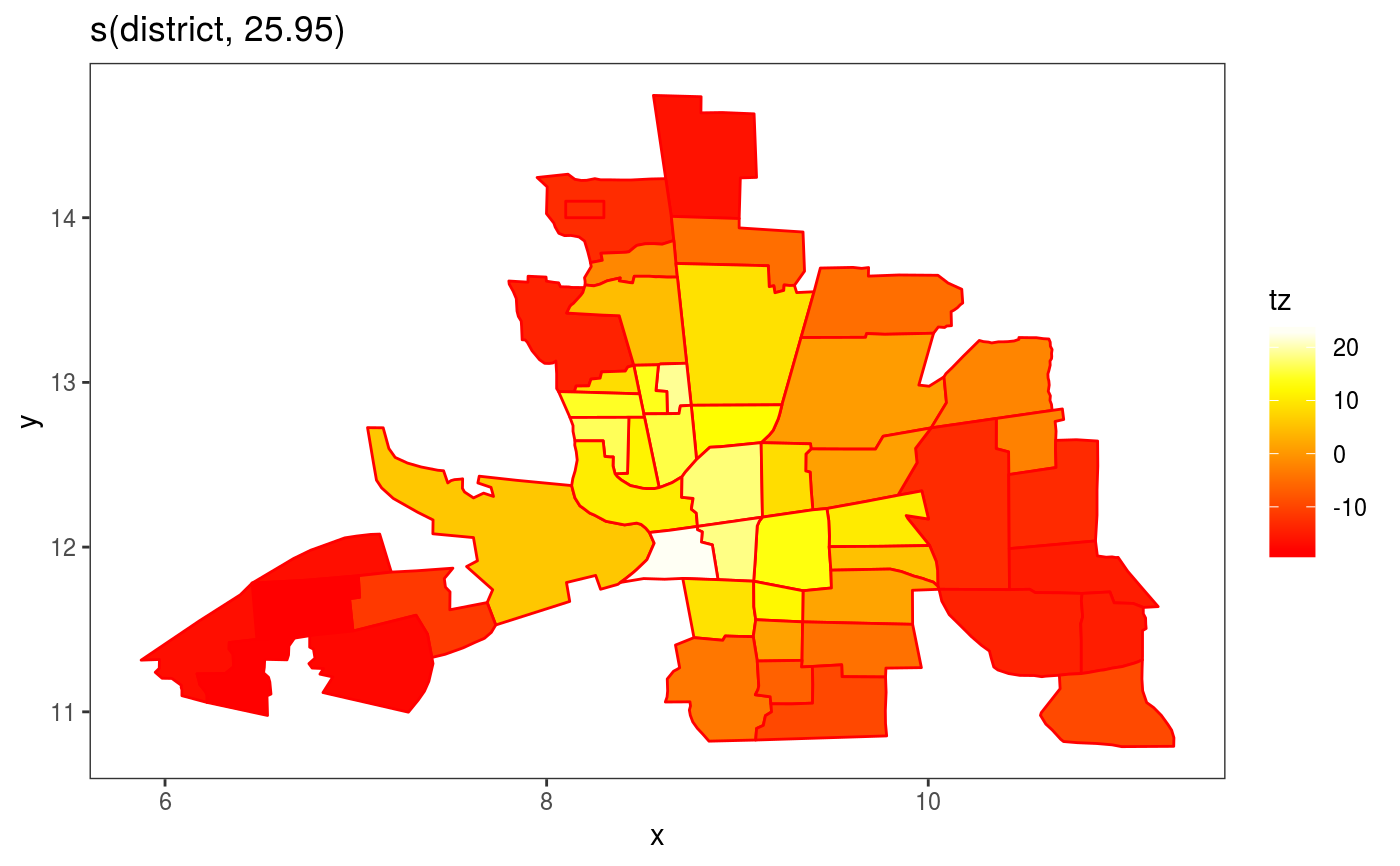
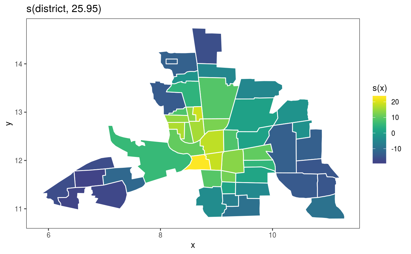
library(mgcViz)
## Load Columbus Ohio crime data (see ?columbus for details and credits)
data(columb)       ## data frame
data(columb.polys) ## district shapes list
xt <- list(polys=columb.polys) ## neighbourhood structure info for MRF
par(mfrow=c(2,2))
## First a full rank MRF...
b <- gam(crime ~ s(district,bs="mrf",xt=xt),data=columb,method="REML")
b <- getViz(b)

# Manual plot
plot(sm(b, 1)) + l_poly(colour = 2) +
  scale_fill_gradientn(colours = heat.colors(50))
#> Scale for 'fill' is already present. Adding another scale for 'fill', which
#> will replace the existing scale.

# Default plot 
plot(b)