Plotting factor or logical parametric effects

These are the plotting methods for parametric factor or logical effects.

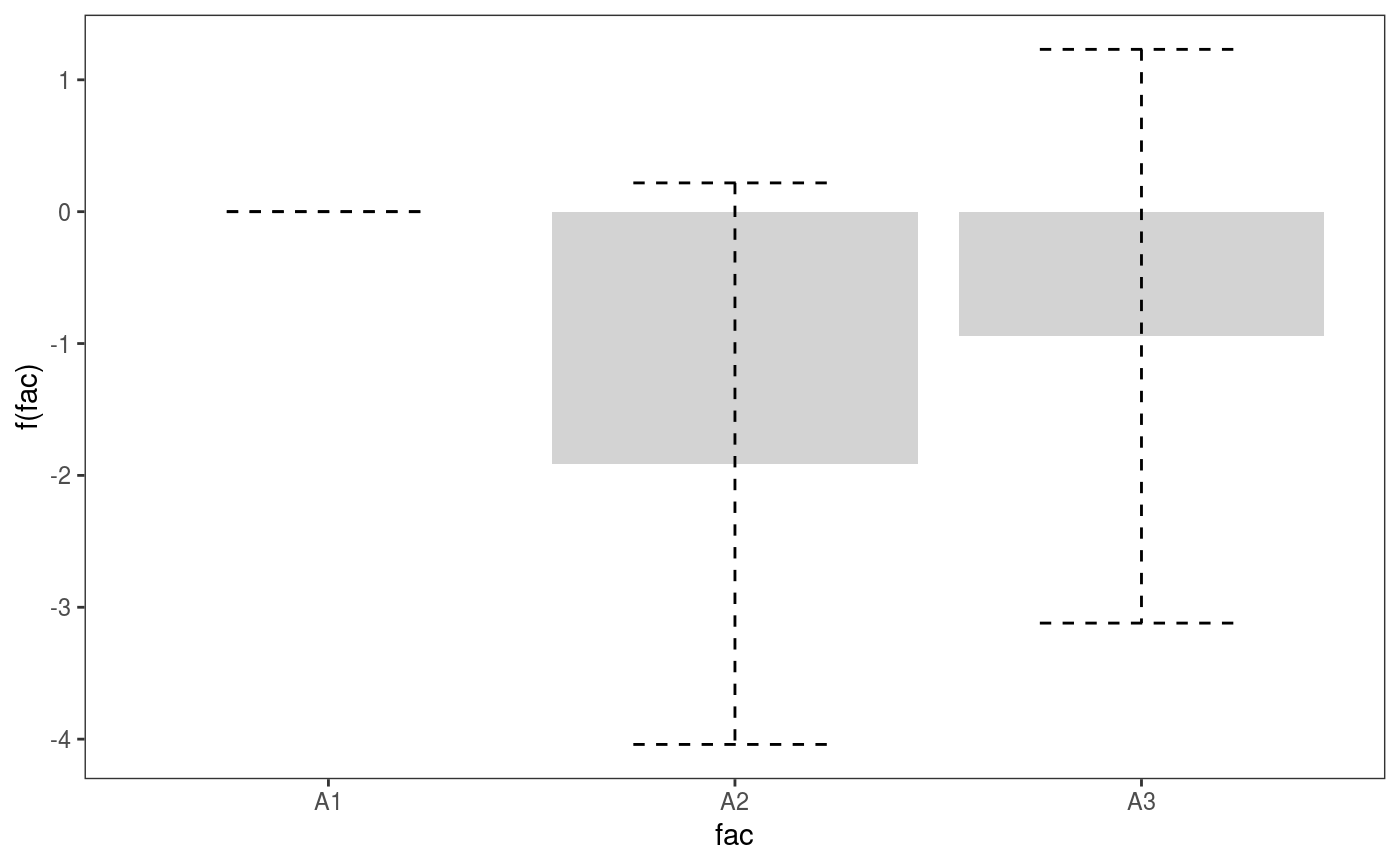
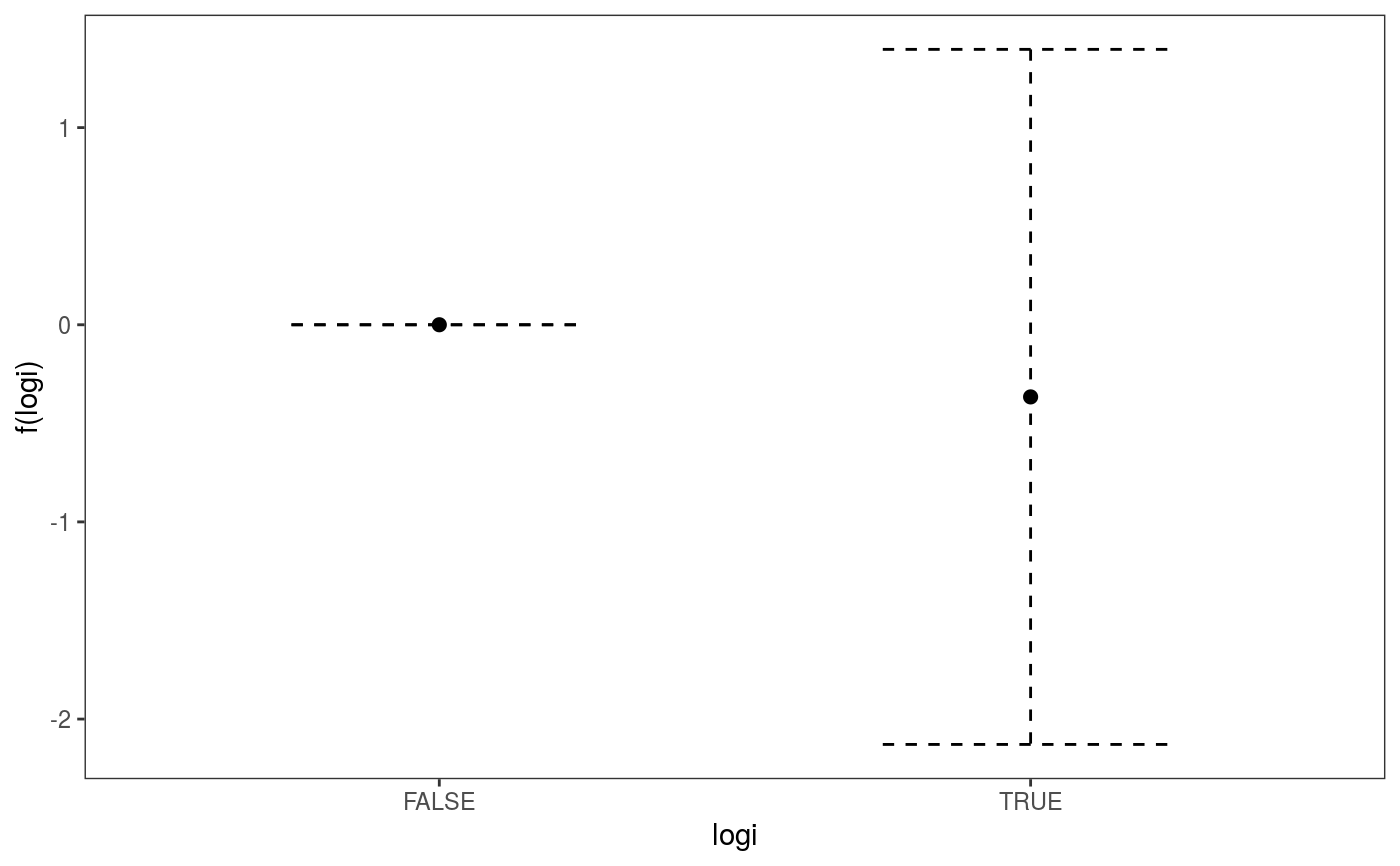
# S3 method for multi.ptermFactor
plot(x, a.facet = list(), asFact = TRUE, ...)

# S3 method for multi.ptermLogical
plot(x, ...)

# S3 method for ptermFactor
plot(x, maxpo = 10000, trans = identity, ...)

# S3 method for ptermLogical
plot(x, maxpo = 10000, trans = identity, ...)

Arguments

x	a factor or logical parametric effect object, extracted using mgcViz::pterm.
a.facet	arguments to be passed to ggplot2::facet_wrap or ggplot2::facet_grid. The former gets called when fix contains one vector, the latter when fix contains two vectors.
asFact	relevant only when working with models fitted with mqgamV. If FALSE quantile of interest (qu) is treated as a continuous variable, otherwise as a factor.
...	currently unused.
maxpo	maximum number of residuals points that will be used by layers such as resRug() and resPoints(). If number of datapoints > maxpo, then a subsample of maxpo points will be taken.
trans	monotonic function to apply to the fit, confidence intervals and residuals, before plotting. Monotonicity is not checked.

Value

An object of class plotSmooth.

Examples

# Simulate data and fit GAM
set.seed(3)
dat <- gamSim(1,n=2000,dist="normal",scale=20)
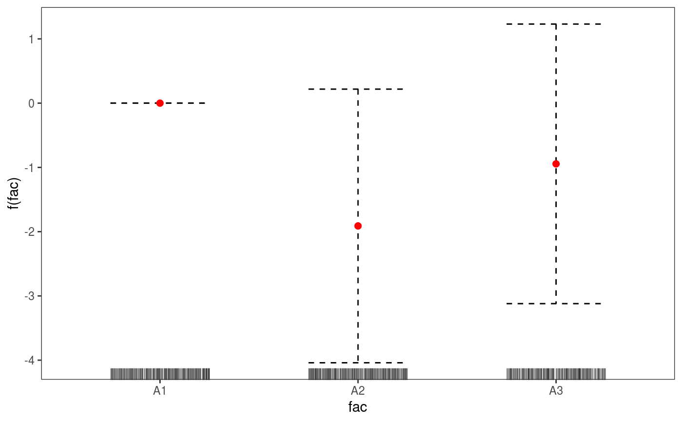
#> Gu & Wahba 4 term additive model
dat$fac <- as.factor( sample(c("A1", "A2", "A3"), nrow(dat), replace = TRUE) )
dat$logi <- as.logical( sample(c(TRUE, FALSE), nrow(dat), replace = TRUE) )
bs <- "cr"; k <- 12
b <- gam(y~fac + s(x0) + s(x1) + s(x2) + s(x3) + logi, data=dat)
o <- getViz(b, nsim = 0)

# Extract factor terms and plot it
pt <- pterm(o, 1)
plot(pt) + l_ciBar() + l_fitPoints(colour = 2) + l_rug(alpha = 0.2)

# Use barplot instead of points
pt <- pterm(o, 1)
plot(pt) + l_fitBar() + l_ciBar()

# Same with binary varible
pt <- pterm(o, 2)
plot(pt) + l_fitPoints() + l_ciBar()