Plotting numeric parametric effects

This is the plotting method for parametric numerical effects.

# S3 method for ptermMatrixNumeric
plot(x, n = 100, xlim = NULL, trans = identity, ...)

# S3 method for multi.ptermNumeric
plot(x, ...)

# S3 method for ptermNumeric
plot(x, n = 100, xlim = NULL, maxpo = 10000, trans = identity, ...)

Arguments

x	a numerical parametric effect object, extracted using mgcViz::pterm.
n	number of grid points used to compute main effect and c.i. lines.
xlim	if supplied then this pair of numbers are used as the x limits for the plot.
trans	monotonic function to apply to the fit, confidence intervals and residuals, before plotting. Monotonicity is not checked.
...	currently unused.
maxpo	maximum number of residuals points that will be used by layers such as resRug() and resPoints(). If number of datapoints > maxpo, then a subsample of maxpo points will be taken.

Value

An object of class plotSmooth.

Examples

# Simulate data and fit GAM
set.seed(3)
dat <- gamSim(1,n=2000,dist="normal",scale=20)
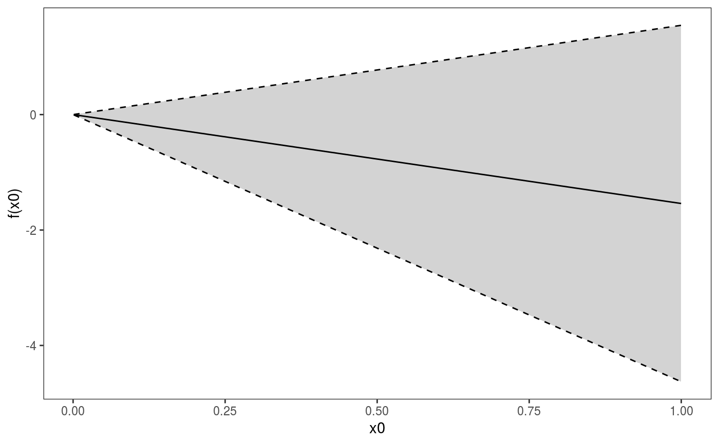
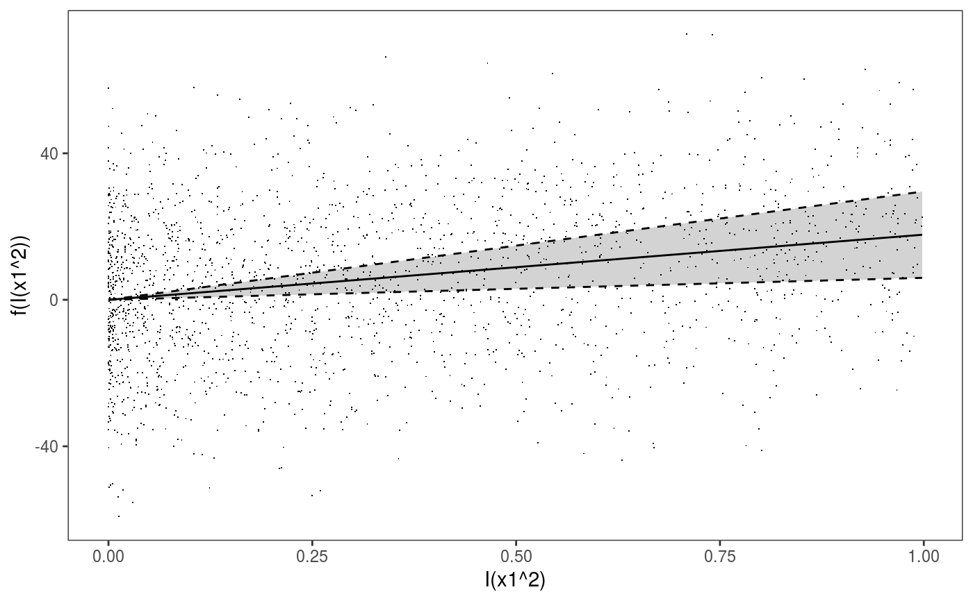
#> Gu & Wahba 4 term additive model
bs <- "cr"; k <- 12
b <- gam(y ~  x0 + x1 + I(x1^2) + s(x2,bs=bs,k=k) +
              I(x1*x2) + s(x3, bs=bs), data=dat)
o <- getViz(b, nsim = 0)

# Extract first terms and plot it
pt <- pterm(o, 1)
plot(pt, n = 60) + l_ciPoly() + l_fitLine() + l_ciLine()

# Extract I(x1^2) terms and plot it with partial residuals
pt <- pterm(o, 3)
plot(pt, n = 60) + l_ciPoly() + l_fitLine() + l_ciLine() + l_points()