QQ plots for gam model residuals

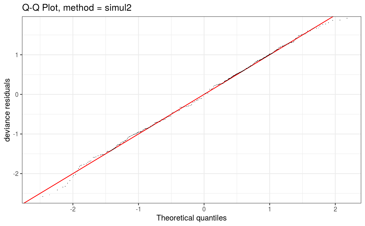
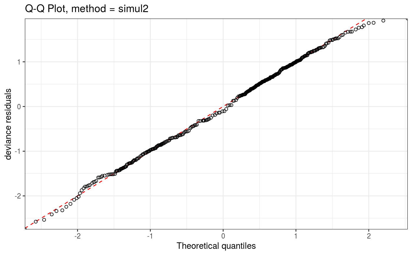
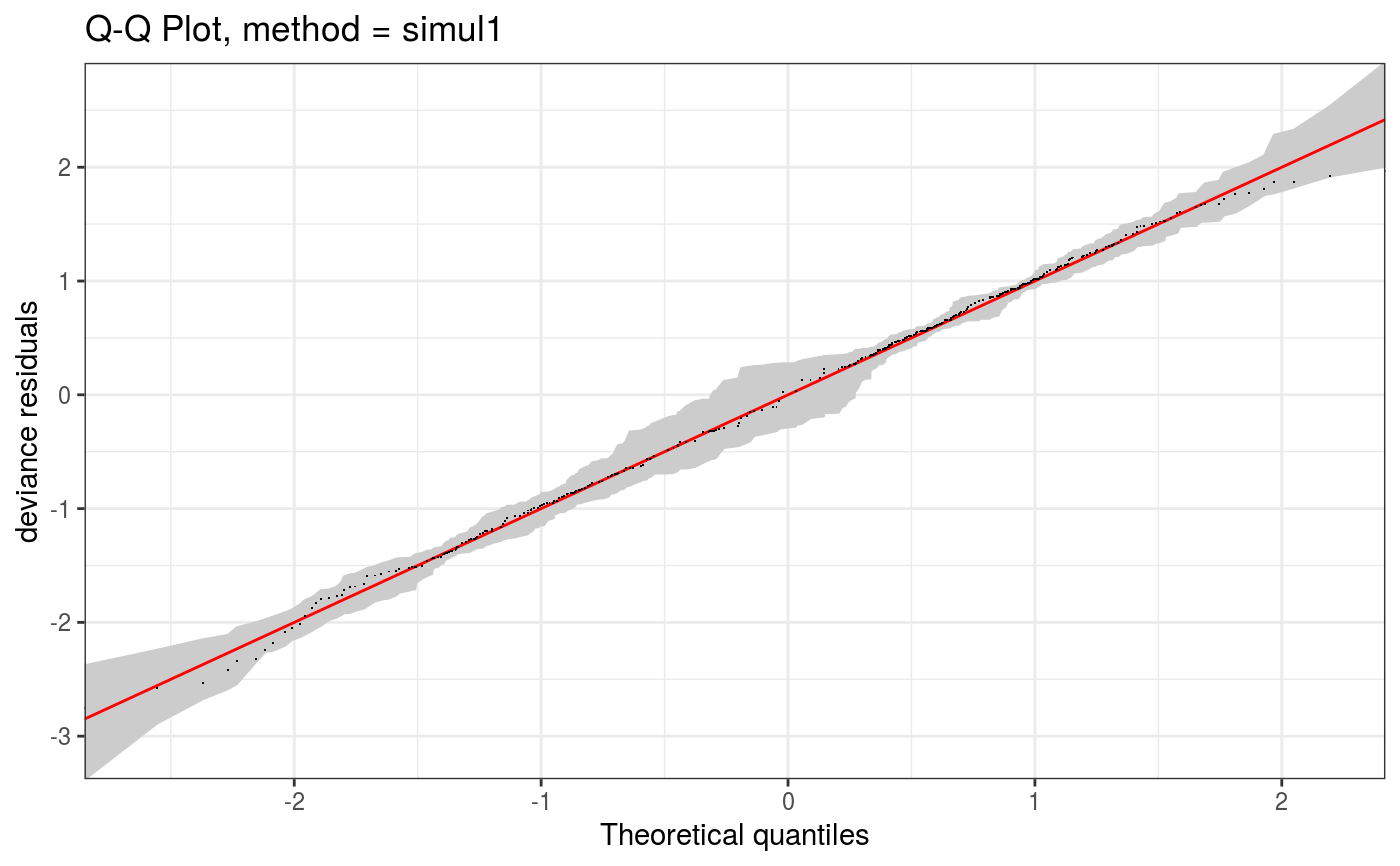
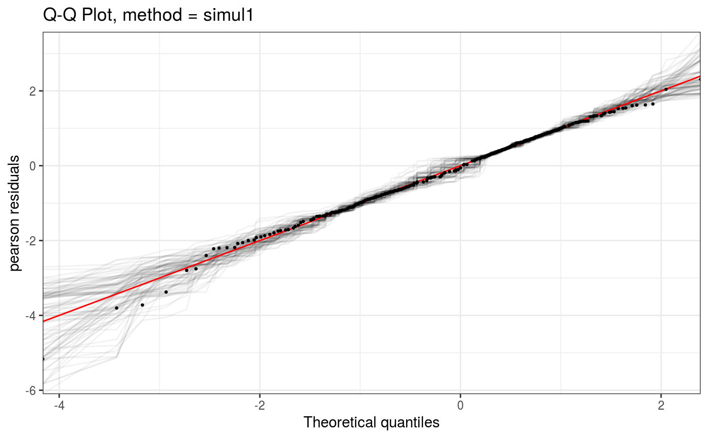
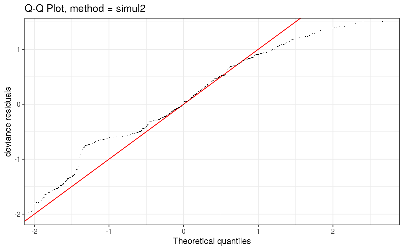
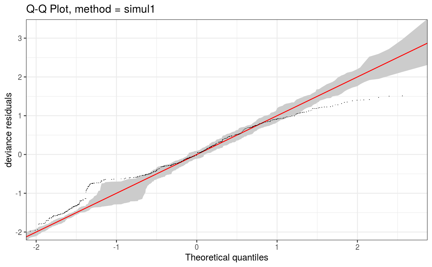
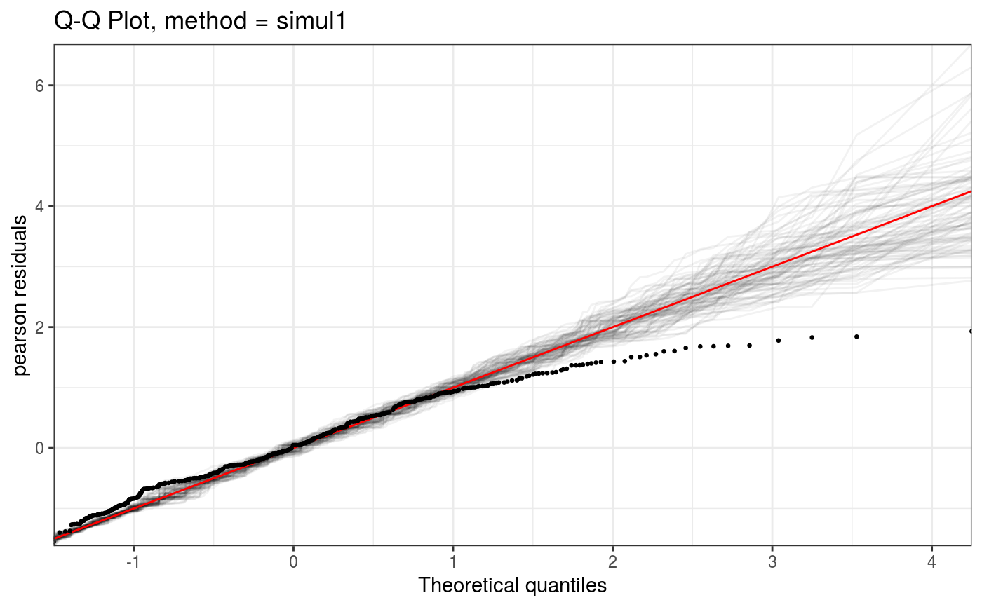
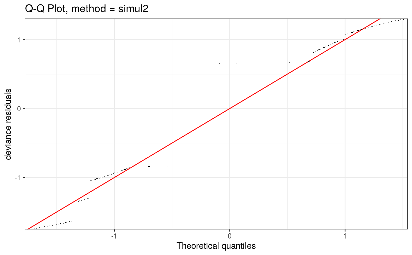
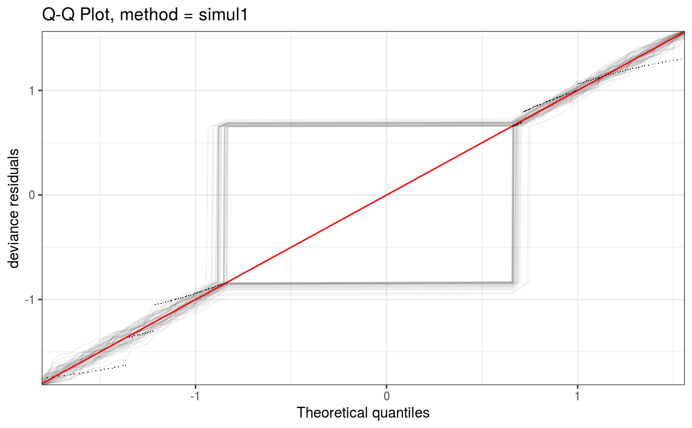
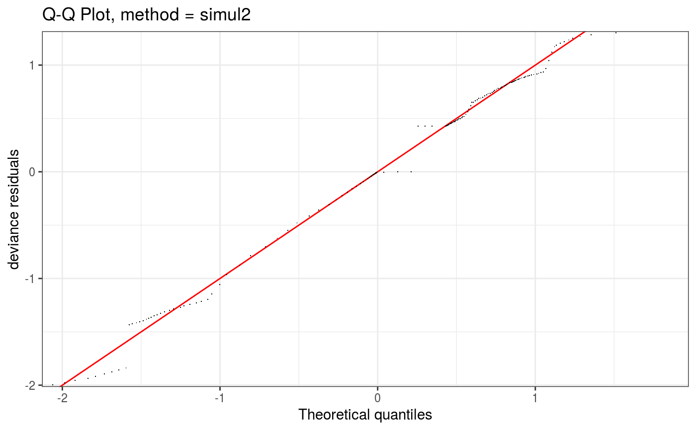
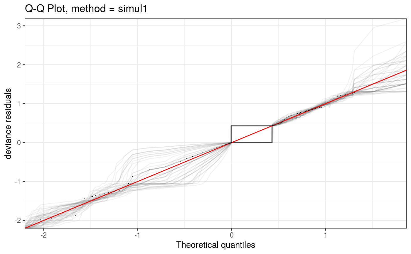
Takes a fitted gam object, converted using getViz, and produces QQ plots of its residuals (conditional on the fitted model coefficients and scale parameter). If the model distributional assumptions are met then usually these plots should be close to a straight line (although discrete data can yield marked random departures from this line).

# S3 method for gamViz
qq(
  o,
  rep = 10,
  level = 0.8,
  method = "auto",
  type = "auto",
  CI = "none",
  worm = FALSE,
  showReps = FALSE,
  sortFun = NULL,
  discrete = NULL,
  ngr = 1000,
  xlim = NULL,
  ylim = NULL,
  a.qqpoi = list(),
  a.ablin = list(),
  a.cipoly = list(),
  a.replin = list(),
  ...
)

Arguments

o	an object of class `gamViz`, the output of a `getViz()` call.
rep	how many replicate datasets to generate to simulate quantiles of the residual distribution. Relevant only if `method` is set to `"simul1"` or `"simul2"`.
level	the level of the confidence intervals (e.g. 0.9 means 90% intervals).
method	the method used to calculate the QQ-plot and, possibly, the confidence intervals. If set to (`"tunif"`) `"tnormal"` the residuals are transformed to (uniform) normal, for which analytic expression for the confidence intervals are available. If set to `"simul1"` or `"simul2"` the theoretical QQ-line is constructed by simulating residuals from the model. Method `"simul2"` does not produce confidence intervals. If set to `"normal"` no simulation or transformation is performed, and a simple normal QQ-plot is produced. If set to `"auto"` the method used to produce the QQ-plot is determined automatically.
type	the type of residuals to be used. See residuals.gamViz.
CI	the type of confidence intervals to be plotted. If set to `"none"` they are not added, if set to `"normal"` they will be based on the assumption that the theoretical quantile distribution is Gaussian and if set to `"quantile"` they will be sample quantiles of simulated responses from the model.
worm	if `TRUE` a worm-plot (a de-trended QQ-plot) is plotted.
showReps	if `TRUE` all the QQ-lines corresponding to the simulated (model-based) QQ-plots.
sortFun	the function to be used for sorting the residuals. If left to `NULL` it will be set to `function(.x) sort(.x, method = "quick")` internally.
discrete	if `TRUE` the QQ-plot is discretized into `ngr` bins before plotting, in order to save plotting time (when the number of observations is large). If left to `NULL`, the discretization is used if there are more than 10^4 observations.
ngr	number of bins to be used in the discretization.
xlim	if supplied then this pair of numbers are used as the x limits for the plot.
ylim	if supplied then this pair of numbers are used as the y limits for the plot.
a.qqpoi	list of arguments to be passed to `ggplot2::geom_point`, which plots the main QQ-plot.
a.ablin	list of arguments to be passed to `ggplot2::geom_abline`, which adds the reference line.
a.cipoly	list of arguments to be passed to `ggplot2::geom_polygon`, which add the confidence intervals.
a.replin	list of arguments to be passed to `ggplot2::geom_line`, which adds a line for each simulated QQ-plot.
...	currently unused.

Value

An object of class c("qqGam", "plotSmooth", "gg").

Details

Here method = "simul1" corresponds to the algorithm described in section 2.1 of Augustin et al. (2012), which involves direct simulations of residuals from the models. This requires o$family$rd to be defined. Setting method = "simul2" results in a cheaper method, described in section 2.2 of Augustin et al. (2012), which requires o$family$qf to be defined.

References

Augustin, N.H., Sauleau, E.A. and Wood, S.N., 2012. On quantile quantile plots for generalized linear models. Computational Statistics & Data Analysis, 56(8), pp.2404-2409.

Examples

######## Example: simulate binomial data
library(mgcViz)
set.seed(0)
n.samp <- 400
dat <- gamSim(1,n = n.samp, dist = "binary", scale = .33)
#> Gu & Wahba 4 term additive model
p <- binomial()$linkinv(dat$f) ## binomial p
n <- sample(c(1, 3), n.samp, replace = TRUE) ## binomial n
dat$y <- rbinom(n, n, p)
dat$n <- n
lr.fit <- gam(y/n ~ s(x0) + s(x1) + s(x2) + s(x3)
              , family = binomial, data = dat,
              weights = n, method = "REML")
lr.fit <- getViz(lr.fit)

# Quick QQ-plot of deviance residuals
qq(lr.fit, method = "simul2")

# Same, but changing points share and type of reference list
qq(lr.fit, method = "simul2",
       a.qqpoi = list("shape" = 1), a.ablin = list("linetype" = 2))

# Simulation based QQ-plot with reference bands 
qq(lr.fit, rep = 100, level = .9, CI = "quantile")

# Simulation based QQ-plot, Pearson resids, all simulations lines shown 
qq(lr.fit, rep = 100, CI = "none", showReps = TRUE, type = "pearson",
       a.qqpoi = list(shape=19, size = 0.5))

### Now fit the wrong model and check
pif <- gam(y ~ s(x0) + s(x1) + s(x2) + s(x3)
           , family = poisson, data = dat, method = "REML")
pif <- getViz(pif)

qq(pif, method = "simul2")

qq(pif, rep = 100, level = .9, CI = "quantile")

qq(pif, rep = 100, type = "pearson", CI = "none", showReps = TRUE,
               a.qqpoi = list(shape=19, size = 0.5))

######## Example: binary data model violation so gross that you see a problem 
######## on the QQ plot
y <- c(rep(1, 10), rep(0, 20), rep(1, 40), rep(0, 10), rep(1, 40), rep(0, 40))
x <- 1:160
b <- glm(y ~ x, family = binomial)
class(b) <- c("gamViz", class(b)) # Tricking qq.gamViz to use it on a glm

# Note that the next two are not necessarily similar under gross 
# model violation...
qq(b, method = "simul2")
qq(b, rep = 50, CI = "none", showReps = TRUE)

### alternative model
b <- gam(y ~ s(x, k = 5), family = binomial, method = "ML")
b <- getViz(b)

qq(b, method = "simul2")
qq(b, rep = 50, showReps = TRUE, CI = "none", shape = 19)

if (FALSE) {
########  "Big Data" example: 
set.seed(0)
n.samp <- 50000
dat <- gamSim(1,n=n.samp,dist="binary",scale=.33)
p <- binomial()$linkinv(dat$f) ## binomial p
n <- sample(c(1,3),n.samp,replace=TRUE) ## binomial n
dat$y <- rbinom(n,n,p)
dat$n <- n
lr.fit <- bam(y/n ~ s(x0) + s(x1) + s(x2) + s(x3)
              , family = binomial, data = dat,
              weights = n, method = "fREML", discrete = TRUE)
lr.fit <- getViz(lr.fit)

# Turning discretization off (on by default for large datasets).
set.seed(414) # Setting the seed because qq.gamViz is doing simulations
o <- qq(lr.fit, rep = 10, method = "simul1", CI = "normal", showReps = TRUE,
            discrete = F, a.replin = list(alpha = 0.1))
o # This might take some time!

# Using default discretization
set.seed(414)
o <- qq(lr.fit, rep = 10, method = "simul1", CI = "normal", showReps = TRUE,
            a.replin = list(alpha = 0.1))
o # Much faster plotting!

# Very coarse discretization
set.seed(414)
o <- qq(lr.fit, rep = 10, method = "simul1", CI = "normal", showReps = TRUE,
            ngr = 1e2, a.replin = list(alpha = 0.1), a.qqpoi = list(shape = 19))
o

# We can also zoom in at no extra costs (most work already done by qq.gamViz)
zoom(o, xlim = c(-0.25, 0.25), showReps = TRUE, discrete = TRUE, a.replin = list(alpha = 0.2))
}

Arguments

Value

Details

References

Examples

Contents