Simulating responses from a GAM object

This method can be used to simulate vectors of responses from a gamObject.

# S3 method for gam
simulate(
  object,
  nsim = 1,
  seed = NULL,
  method = "auto",
  newdata,
  u = NULL,
  w = NULL,
  offset = NULL,
  trans = NULL,
  ...
)

Arguments

object	the output of a gam() or bam() call.
nsim	the number of simulated vectors of responses. A positive integer.
seed	currently not used.
method	the method used for the simulation. If set to "rd" then o$family$rd() will be used, if available. If set to "qf" then o$family$qf() (which is the inverse cdf of the response distribution) will be used to transform some uniform variates.
newdata	Optional new data frame or list to be passed to predict.gam.
u	a matrix where each row is a vector of uniform random variables in (0, 1). This will be used to simulate responses only if method = "qf".
w	vector of prior weights to be used in the simulations. If newdata==NULL then w is set to object$prior.weights otherwise it is a vector of ones.
offset	numeric vector of offsets. For GAMs with multiple linear predictor (see eg gaulss) it must be a list of vectors. NB: if newdata!=NULL the offsets will be assumed to be zero, unless their are explicitly provided. If newdata==NULL then simulations will use the offsets used during model fitting, and offset argument will be ignored.
trans	function used to transform or summarize each vector of simulated responses. It must take a vector as argument, but it can output a vector or a scalar. Potentially useful for saving storage (e.g. by transforming each simulated vector to a scalar). If left to NULL then trans = identity will be used.
...	currently not used.

Value

A matrix where each row is a vector of simulated responses. The number of columns is equal to the number of responses in the fitted object.

Examples

library(mgcViz)

set.seed(2) ## simulate some data... 
dat <- gamSim(1,n=400,dist="normal",scale=2)
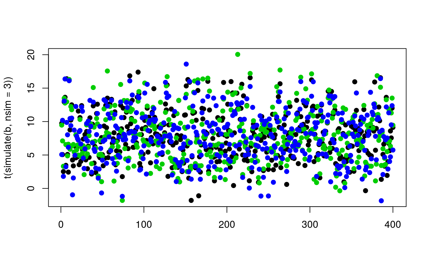
#> Gu & Wahba 4 term additive model
b <- gam(y~s(x0)+s(x1)+s(x2)+s(x3),data=dat)

# Simulate three vectors of responses
matplot(t(simulate(b, nsim = 3)), pch = 19, col = c(1, 3, 4))