2. Exercises on chaotic maps and kernel regression smoothing

Simulation based inference on the Ricker model
Adaptive kernel regression smoothing

Simulation based inference on the Ricker model

Here we consider an extremely simple model for population dynamics, the Ricker map: \[ y_{t+1} = ry_te^{-y_t}, \] where \(y_t>0\) represents the size of the population at time \(t\) and \(r>0\) is its growth rate. The model can show a wide range of dynamics, depending on the value of \(r\). A simple function for generating a trajectory from the map is the following:

rickerSimul <- function(n, nburn, r, y0 = 1){

 y <- numeric(n)
 yx <- y0
 
 # Burn in phase
 if(nburn > 0){
   for(ii in 1:nburn){ 
     yx <- r * yx * exp(-yx)
   }
 }
 
 # Simulating and storing
 for(ii in 1:n){
  yx <- r * yx * exp(-yx)
  y[ii] <- yx
 }
 
 return( y )
}

where:

y0 is the initial population size;
n is the total number of time steps to be stored;
nburn is the initial number of simulations that are discarded before storing the following n iterations.

Q1 start: create a C version of rickerSimul and compare its speed with that of its R version. To do this you will need a C version of exp(), which you can get by including the Rmath.h header Q1 end.

Suppose that we observe some noisy data from the map, that is we observe: \[ z_t = y_t e^{\epsilon_t}, \;\;\; \text{with} \;\; \epsilon_t \sim N(0, \sigma^2), \] In particular, assume that we have observed a data set simulated as follows:

nburn <- 100
n <- 50

y0_true <- 1
sig_true <- 0.1
r_true <- 10

Ntrue <- rickerSimul(n = n, nburn = nburn, r = r_true, y0 = y0_true)
yobs <- Ntrue * exp(rnorm(n, 0, sig_true))

plot(yobs, type = 'b')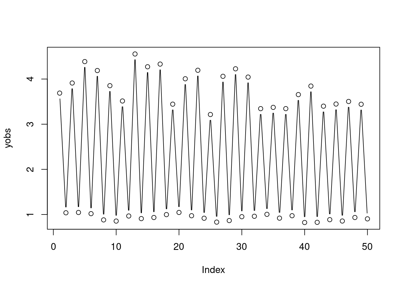

Q2 start: build a C function for calculating the likelihood of the data. You will need the function

dnorm(double, double, double, int);

which is defined in the Rmath.h header. Its arguments are the same as those of the dnorm function in R (see ?dnorm). Wrap your C likelihood function into an R function, e.g.

myLikR <- function(logr, logsig, logy0, yobs, nburn){
  n <- length(yobs)
  r <- exp(logr)
  sig <- exp(logsig)
  y0 <- exp(logy0)
  
  ysim <- .Call("rickerSimul_C", n, nburn, r, y0)
  
  llk <- .Call("rickerLLK_C", yobs, ysim, sig)
  
  return( llk )
  
}

and use it within a Metropolis-Hastings algorithm to sample the posterior of \(\log(r)\), \(\log(\sigma)\) and \(\log(y_0)\) (e.g. using the metrop function in the mcmc package). We work with the log-variables to enforce positivity. Does the marginal posterior distribution of the three parameters look fine? In particular, is the posterior for \(y_0\) very dispersed? Try to explain what is going on Q2 end.

Now, assume that the observed data has been simulated as follows:

r_true <- 44

Ntrue <- rickerSimul(n = n, nburn = nburn, r = r_true, y0 = y0_true)
yobs <- Ntrue * exp(rnorm(n, 0, sig_true))

plot(yobs, type = 'b')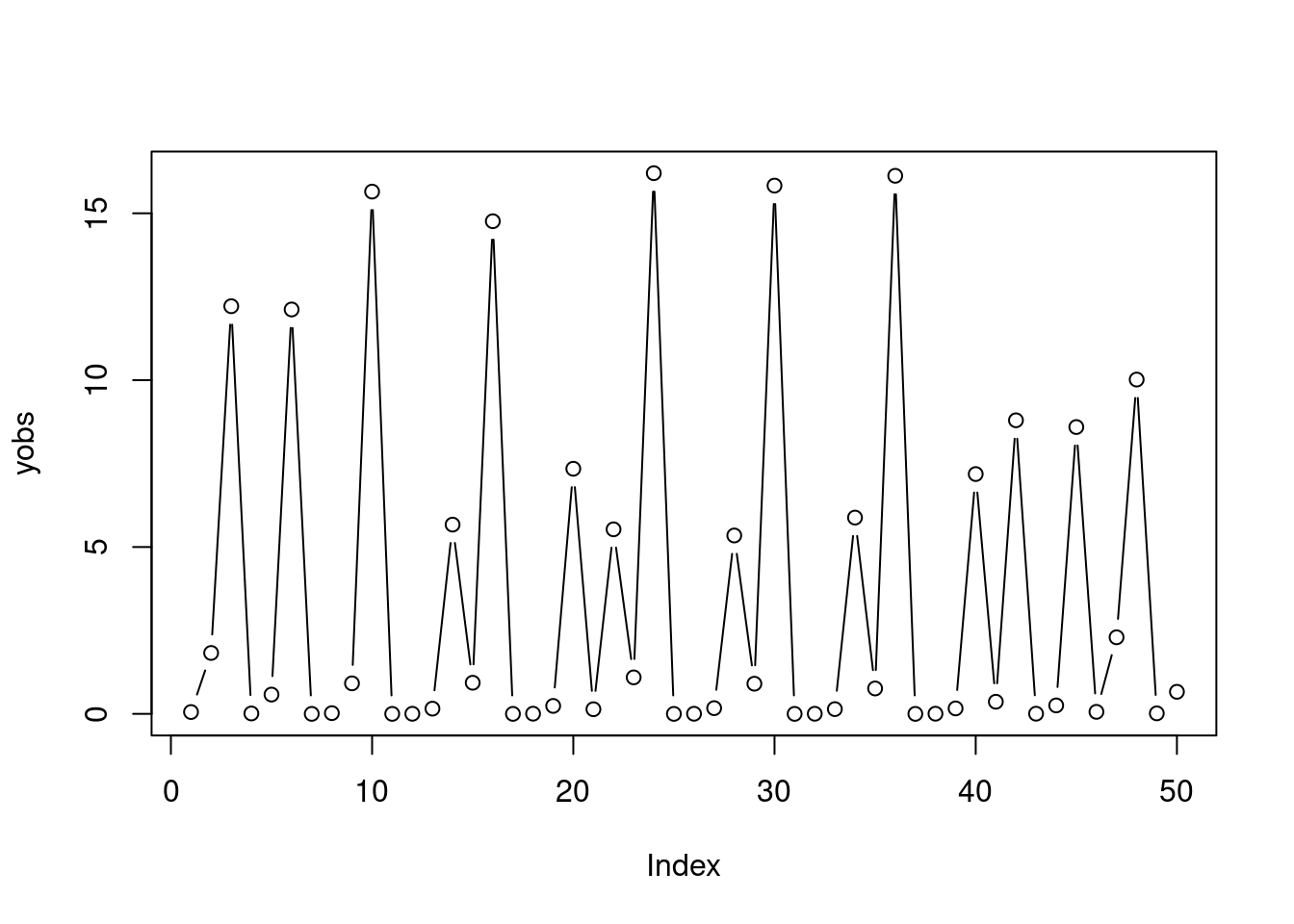

Q3 start: try to use Metropolis-Hastings again to sample from the posterior under the new data, are you encountering any problem? If so, try to look at slices of the likelihood w.r.t. each parameter of the model, while keeping the remaining parameters fixed to their true value. Does the likelihood look nice and smooth? What do you think it’s happening? Q3 end.

From the previous question you should have observed that the slices of the likelihood w.r.t. \(r\) look horrible for \(r\) greater than around 12. Hence, the MH algorithm does not mix. The reason for this behaviour is that the system is chaotic for high \(r\), and the simulated trajectory become highly sensitive to small perturbations of \(r\) or of \(y_0\). To simplify things, assume that we know the true value of \(\sigma\) and that we do not care about the value of the initial value \(y_0\). In particular, let us just assume that is \(y_0\) a random variable (rather than an unknown parameter) in our model, distributed according to \(y_0 \sim \text{Unif}(1, 10)\) (for example). One way of working around the chaotic behaviour of the Ricker map is to build a new likelihood based a new set of summary statistics of the raw data, whose distribution varies smoothly (rather than chaotically) with \(r\).

In particular, consider the sample mean \(s_1\) and standard deviation \(s_2\) of the observed data, \(z_1, \dots, z_n\). For simplicity, assume that these two statistics are independently normally distributed, that is \[ s_1 \sim \text{N}(\mu_1, \tau_1^2), \;\;\; s_2 \sim \text{N}(\mu_2, \tau_2^2), \] with \(\text{cov}(s1, s2) = 0\). Hence, the likelihood of the observed statistics, \(p(s_1, s_2|r)\), is just the product of two normal densities, whose means and variances (\(\mu_1\), \(\mu_2\), \(\tau_1\) and \(\tau_2\)) are unknown functions of \(r\). To sample the posterior corresponding to \(p(s_1, s_2|r)\), we need to be able to estimate this likelihood for any fixed \(r\). This can be achieved by simulation, using the following function:

synllk <- function(logr, nsim){
  
  r <- exp(logr)
  s1 <- s2 <- numeric(nsim)
  y0 <- runif(nsim, 1, 10)
  
  # Note: sigma is assumed to be known!
  for(ii in 1:nsim){
    ysim <- rickerSimul(n = n, nburn = nburn, r = r, y0 = y0[ii]) * exp(rnorm(n, 0, sig_true))
    s1[ii] <- mean(ysim)
    s2[ii] <- sd(ysim)
  }
  
  out <- dnorm(mean(yobs), mean(s1), sd(s1), log = TRUE) + 
         dnorm(sd(yobs), mean(s2), sd(s2), log = TRUE)
  
  return( out )
}

For a given value of \(\log{r}\), we estimate \(\mu_1\), \(\mu_2\), \(\tau_1\) and \(\tau_2\) by simulating nsim trajectories from the model, and then we evaluate the log-likelihood based on such estimates.

Q4 start: try to run a MH algorithm to (approximately) sample the posterior \(p(r|s_1, s_2)\), using the synllk. You should get better mixing than under the full posterior \(p(y_1, \dots, y_n|r)\). But synllk is very slow, so try to implement it in C, and compare your C version with the R version above in terms of computing time. You can also try to use different statistics than those used above. If you don’t know how to generate random variables in C, you can simply generate them in R and then pass them to your C function Q4 end.

Q5 start: By now, you should have implemented C versions of the rickerSimul and of the synllk functions. If you have time, write also a C version of the basic Metropolis-Hastings algorithm, so that you are able to do the whole thing in C Q5 end.

Adaptive kernel regression smoothing

Consider data generated from the following model \[ y_i = \sin(\alpha\pi x^3) + z_i, \;\;\; \text{with} \;\;\; z_i \sim ~ \text{N}(0, \sigma^2) \] for \(i = 1, \dots, n\). Below we simulate some data from this model, with \(\alpha = 4\), \(\sigma = 0.2\) and \(n = 200\):

set.seed(998)
nobs <- 200 
x <- runif(nobs)
y <- sin(4*pi*x^3) + rnorm(nobs, 0, 0.2)
plot(x, y)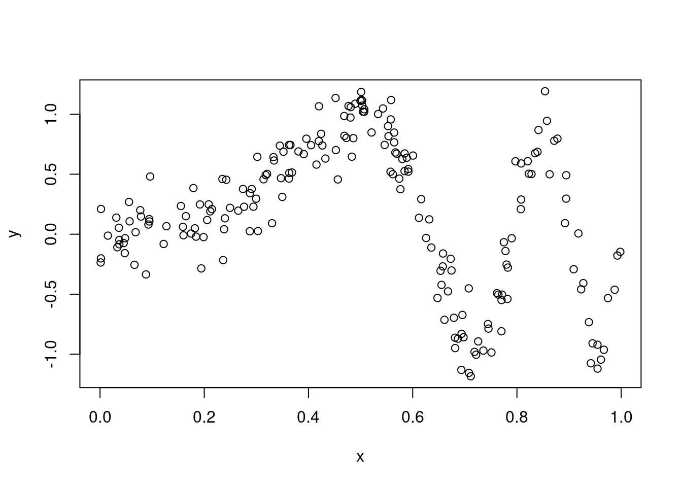

Now, suppose that we want to model this data using a kernel regression smoother (KRS). That is, we want to estimate the conditional expectation \(\mu(x)=\mathbb{E}(y|x)\) using \[ \hat{\mu}(x) = \frac{\sum_{i=1}^n\kappa_\lambda(x, x_i)y_i}{\sum_{i=1}^n\kappa_\lambda(x, x_i)} \] where \(\kappa\) is a kernel with bandwidth \(\lambda > 0\). The function below computes this estimator by adopting a Gaussian kernel with variance \(\lambda^2\):

meanKRS <- function(y, x, x0, lam){

 n <- length(x)
 n0 <- length(x0)
 
 out <- numeric(n0)
 for(ii in 1:n0){
  out[ii] <- sum( dnorm(x, x0[ii], lam) * y ) / sum( dnorm(x, x0[ii], lam) )   
 }
 
 return( out )
}

We now use it to produce two fits, obtained using different values of \(\lambda\):

xseq <- seq(0, 1, length.out = 1000)
muSmoothLarge <- meanKRS(y = y, x = x, x0 = xseq, lam = 0.06)
muSmoothSmall <- meanKRS(y = y, x = x, x0 = xseq, lam = 0.02)
plot(x, y, col = "grey")
lines(xseq, muSmoothLarge, col = 2)
lines(xseq, muSmoothSmall, col = 4)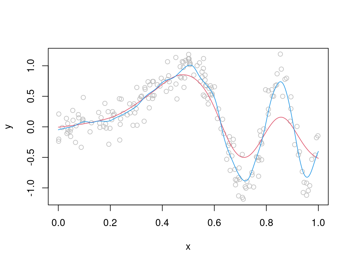

Q1a start: Produce a C version of meanKRS and compare its computational performance with that of the R version above. You will need the function

dnorm(double, double, double, int);

which is defined in the Rmath.h header. Its arguments are the same as those of the dnorm function in R (see ?dnorm) Q1a end.

Q1b start (Optional) In practice, we don’t want to select \(\lambda\) manually and using \(k\)-fold cross validation is generally preferable. Hence, create a cross-validation routine for selecting \(\lambda\), implement it in C and compare its computing time with its R version. Are the gains in performance comparable to those that you got by implementing meanKRS in C? Q1b start

From the plot above, it should be clear that no single value of \(\lambda\) will lead to a satisfactory fit. The basic problem is that the true \(\mu(x)\) is smooth for \(x < 0.5\) and quite wiggly for \(x > 0.5\), hence setting \(\lambda\) to a high (low) value will produce a good fit in the first (second) interval and a bad fit in the second (first). To solve this issue, we should really let the smoothness depend on \(x\), that is we need to \(\lambda = \lambda(x)\). A simple way of doing this is the following:

fit the KRS model as before with some fixed value of \(\lambda\);
let the residuals from the first model be \(r_1, \dots, r_n\);
estimate their expected absolute value \(v(x)=\mathbb{E}(|r||x)\) using another KRS model with the same \(\lambda\);
let the resulting estimates be \(\hat{v}(x_1), \dots, \hat{v}(x_n)\);
fit another KRS model to the original data using: \[ \hat{\mu}(x) = \frac{\sum_{i=1}^n\kappa_{\lambda_i}(x, x_i)y_i}{\sum_{i=1}^n\kappa_{\lambda_i}(x, x_i)} \] where \(\lambda_i = \lambda \tilde{w}_i\) with \(\tilde{w}_i = n w_i / \sum_{i=1}^n w_i\) (so that the weights sum to \(n\)) and \(w_i = 1/\hat{v}(x_i)\).

The rationale is that we start with a standard KRS with fixed \(\lambda\) determined, for instance, by cross-validation. Then we model the residuals of that model to see where, along \(x\), our fit should have been more flexible. In particular, in the final model we use fit using larger bandwidth where the residuals where larger (in absolute value). The whole procedure is implemented by this function:

mean_var_KRS <- function(y, x, x0, lam){

 n <- length(x)
 n0 <- length(x0)
 mu <- res <- numeric(n) 
   
 out <- madHat <- numeric(n0)
 
 for(ii in 1:n){
  mu[ii] <- sum( dnorm(x, x[ii], lam) * y ) / sum( dnorm(x, x[ii], lam) )   
 }
 
 resAbs <- abs(y - mu)
 for(ii in 1:n0){
  madHat[ii] <- sum( dnorm(x, x0[ii], lam) * resAbs ) / sum( dnorm(x, x0[ii], lam) )   
 }
 
 w <- 1 / madHat
 w <- w / mean(w)
 
 for(ii in 1:n0){
  out[ii] <- sum( dnorm(x, x0[ii], lam * w[ii]) * y ) / 
             sum( dnorm(x, x0[ii], lam * w[ii]) )   
 }
 
 return( out )
}

As you can see this leads to a better fit:

xseq <- seq(0, 1, length.out = 1000)
muSmoothAdapt <- mean_var_KRS(y = y, x = x, x0 = xseq, lam = 0.06)
plot(x, y, col = "grey")
lines(xseq, muSmoothLarge, col = 2) # red
lines(xseq, muSmoothSmall, col = 4) # blue
lines(xseq, muSmoothAdapt, col = 1) # black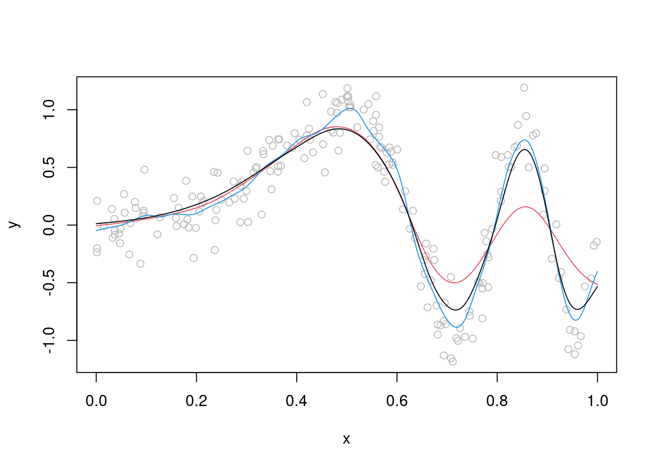

Q2 start: Produce a C version of mean_var_KRS, possibly including a cross-validation routine for \(\lambda\) also implemented in C, and compare its computational performance with that of the R version. Do you think that the adaptive smoother produced here would work well under heteroscedasticity? Q2 end