Computing the c.d.f. of the Tweedie distribution

Here we consider the Tweedie distribution which includes continuous distributions, such as the normal and gamma, and discrete distributions, such as the Poisson. Its density is \[ p(y|\mu,\phi,p)=a(y,\phi,p)\exp\bigg[\frac{1}{\phi}\{y\theta-\kappa(\theta)\}\bigg], \] where \[ \theta=\frac{\mu^{1-p}}{1-p}\;\;\text{for}\;p\neq1\;\;\;\text{and}\;\;\;\theta=\log\mu\;\;\text{for}\;p=1, \] and \[ \kappa(\theta)=\frac{\mu^{2-p}}{2-p}\;\;\text{for}\;p\neq2\;\;\;\text{and}\;\;\;\theta=\log\mu\;\;\text{for}\;p=2. \] with \(\mu>0\) being the mean, \(\phi>0\) the scale and \(1\leq p\leq2\) is such that \(\text{var}(y)=\mu^{p}\). As explained in Dunn and Smyth (2005), evaluating the Tweedie density requires approximating the factor \(a(y,\phi,p)\), which does not have a closed-form expression, using specifically designed numerical methods. Here we consider the simpler problem of numerically approximating the Tweedie c.d.f. \(P(y|\mu,\phi,p)\), under the assumption that \(a(y,\phi,p)\) is unknown.

For \(1\leq p\leq2\), a Tweedie variable \(y\) can be written as the sum of \(N\) i.i.d. Gamma distributed random variables \(z_{1},\dots,z_{N}\) with shape \(-\alpha\) and scale \(\gamma\) (hence with mean \(-\alpha\gamma\) and variance \(-\alpha\gamma^{2}\)), while \(N\) follows a Poisson distribution with rate \(\lambda\). In terms of the original Tweedie parameters, we have \[ \lambda=\frac{\mu^{2-p}}{\phi(2-p)}, \;\;\; \alpha=(2-p)/(1-p) \;\;\; \text{and} \;\;\; \gamma=\phi(p-1)\mu^{p-1}. \] So, if \(p_{G}\) indicates the c.d.f. of a Gamma distribution with parameters \(-k\alpha\) and \(\gamma\), \(p_{p}\) is the p.m.f. of a Poisson with rate \(\lambda\) and we indicate with \(p(Y < y)\) the Tweedie c.d.f., we have \[ p(Y<y)=p\Big(\sum_{i=1}^{N}z_{i}<y\Big)=\sum_{k=1}^{\infty}p_{G}\Big(\sum_{i=1}^{k}z_{i}<y\Big)p_{P}(N=k), \] where the second equality holds due to the Law of Total Probability. Now, we want to avoid computing that infinite sum, hence we approximate it by \[ p(Y<y)\approx\hat{p}(Y<y)=\sum_{k=k_{min}}^{k_{max}}p_{G}\Big (\sum_{i=1}^{k}z_{i}<y \Big )p_{P}(N=k), \] for some \(k_{min}\) and \(k_{max}\).

How to choose \(k_{min}\) and \(k_{max}\)? Given that \(p_{P}\) is maximal at \(k = \text{floor}(\lambda)\), and then monotonically decreases as we move \(k\) away from the mode, a reasonable approach is to choose \(k_{min}\) and \(k_{max}\) such that \(p_{P}(N=k) < \epsilon p_{P}\{N=\text{floor}(\lambda)\}\) for \(k<k_{min}\) or \(k>k_{max}\), for some small \(\epsilon\). If we do so, it is clear that the a very pessimistic bound on the absolute approximation error is \[ |p(Y<y)-\hat{p}(Y<y)| < p_{P}(N<k_{min} \; \text{or} \; N>k_{max}) = 1 - p_{P}(k_{min}<N<k_{max}), \] which is easy to compute. Of course, \(k_{min}\) and \(k_{max}\) are not known in advance, but we can initialize \(k\) to \(\text{floor}(\lambda)\) and then increase \(k\) until we get to \(p_{P}(N=k) < \epsilon p_{P}\{N=\text{floor}(\lambda)\}\), which means that we have found \(k_{max}\). Then we can set \(k\) to the Poisson mode and decrease \(k\) until we find \(k_{min}\). All this is implemented in the following R function:

pTweedR0 <- function(y, mu, phi, p, eps = 1e-17, log = FALSE){
  
  # Get param lambda, gamma and alpha to be used in gamma and poisson distrib
  la <- mu^(2-p) / ( phi * (2-p) )
  ga <- phi * (p-1) * mu^( p-1 )
  al <- (2-p) / ( 1-p )
  
  # Mode of Poisson is at k = floor(lambda). 
  # If mode is 0, we start from 1 instead.
  k0 <- max(floor(la), 1)
  
  # Poisson density at its mode
  mxlpP <-  dpois(k0, la)
  
  # Get probability contribution at Poisson mode
  pTw <- mxlpP * pgamma(y, shape = - k0 * al, scale = ga)
  
  # Initialize k at mode
  k <- k0 
  lP <- mxlpP
  
  # Sum from mode k = floor(lambda) upward until we find kmax
  while ( lP > mxlpP * eps ){
    k <- k + 1
    lP <- dpois(k, la)
    pTw <- pTw + lP * pgamma(y, shape = - k * al, scale = ga)
  }
  kmax <- k
  
  # Reset k to the Poisson mode, and now go down until we find kmin
  k <- k0
  lP <- mxlpP
  while ( lP > mxlpP * eps && k > 0  ){
    k <- k - 1
    lP <- dpois(k, la)
    pTw <- pTw + lP * pgamma(y, shape = - k * al, scale = ga)
  }
  kmin <- k
  
  if( log ) { pTw <- log( pTw ) }
  
  return( pTw )
  
}

Having defined a function for approximating the Tweedie c.d.f., we need to verify whether it is correct. Given that the true c.d.f. is unknown, we compare our function with the ptweedie function from the tweedie package. Below, we simulate a random vector of Tweedie parameters, and then we compare the (log) c.d.f.s produced by pTweedR0 with those obtained using ptweedie:

library("tweedie")
nsim <- 1e3
mu <- runif(nsim, 0, 10)
phi <- 0.01 + rexp(nsim, 1)
p <- runif(nsim, 1.001, 1.999)

lpr1 <- lpr2 <- rep(NA, nsim)
for(ii in 1:nsim){
  y <- rtweedie(n = 1, mu = mu[ii], phi = phi[ii], power = p[ii])
  lpr1[ii] <- pTweedR0(y = y, mu = mu[ii], phi = phi[ii], p = p[ii], log = TRUE)
  lpr2[ii] <- log(ptweedie(q = y, mu = mu[ii], phi = phi[ii], power = p[ii]))
}

par(mfrow = c(1, 2))
plot(lpr1, lpr2, xlab = "pTweedR0", ylab = "ptweedie") 
abline(0, 1)
plot(lpr1 - lpr2, ylab = "pTweedR0 - ptweedie") 
abline(h = 0)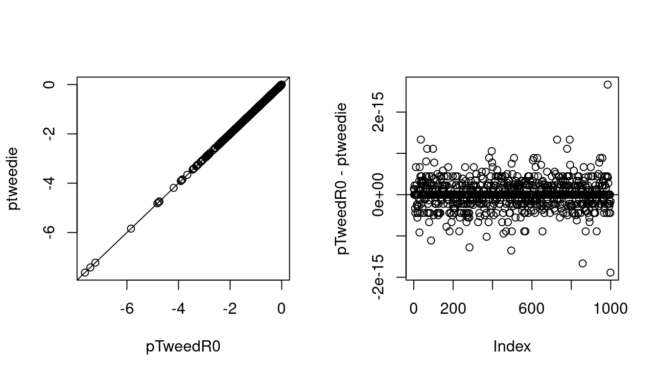

The log c.d.f.s are very close, why is not surprising as ptweedie uses pretty much the same approximation we are using.

Q1 start: The pTweedR0 function requires explicitly looping in R, because \(k_{min}\) and \(k_{max}\) are not known in advance but must be determined iteratively. To address this, create an Rcpp version of pTweedR0 and compare its computational performance with that of pTweedR0 Q1 end.

Q2 start: Most the function provided by R for evaluating the c.d.f. of a random variable (e.g. pnorm(), pexp()) are vectorized in all their main arguments (e.g. pnorm() is vectorized in the arguments q, mean and sd). Our pTweedR0 function cannot be not vectorized directly, because \(k_{min}\) and \(k_{max}\) depend on \(y\) and on the Tweedie parameters. Use Rcpp to create a vectorized C++ version of pTweedR0 (that is a version of pTweedR0 with accepts vector inputs for y, mu, phi and p) and compare its performance with that of simply using pTweedR0 within a for() loop in R Q2 end.