3. Example on multivariate KDE with RcppArmadillo
Introduction
To provide a more challeging example illustrating the capabilities of RcppArmadillo, here we show how to perform multivariate kernel density estimation (k.d.e.) using this library. In particular, let \({\bf x}_1^o, \dots, {\bf x}_n^o\) be \(d\)-dimensional vectors, sampled from the density \(\pi(\bf x)\). A k.d.e. estimate of \(\pi({\bf x})\) is
\[
\hat{\pi}_{\bf H}({\bf x}) = \frac{1}{n} \sum_{i=1}^n \kappa_{\bf H}({\bf x} - {\bf x}_i^o),
\]
where \(\kappa_{\bf H}\) is a kernel with positive definite bandwidth matrix \({\bf H}\). Here we assume that \(\kappa_{\bf H}\) is a multivariate Gaussian kernel, with covariance matrix \({\bf H}\). Further, the data is generated from the mixture of warped Gaussians of Fasiolo et al. (2018). The details of this density are unimportant here, what matters is that the example is defined in \(d>2\) dimensions and, under such a density \(\pi({\bf x})\), the joint distribution of the first two dimensions is far from Gaussian while the remaining dimensions are standard i.i.d. Gaussian variables.
Samples from this density can be generated using the following functions:
rBanana <- function(n, d, a, b, shi1, shi2){
  out <- matrix(rnorm(d*n), n, d);
  out[ , 1] <- out[ , 1] * a
  out[ , 2] <- out[ , 2] - b * (out[ , 1]^2 - a^2)
  out[ , 1] <- out[ , 1] + shi1
  out[ , 2] <- out[ , 2] + shi2
  return( out )
}

rBanMix <- function(n, d, w, a, b, shi1, shi2){
  nmix <- length( a );
  m <- floor( n * w );
  m[1] <- m[1] + n - sum(m);
  m <- round(m);
  out <- lapply(1:nmix, function(.ii)
                         rBanana(m[.ii], d, a[.ii], b[.ii], shi1[.ii], shi2[.ii])
               )
  out <- do.call("rbind", out)
  return( out );
}
which we use here to generate \(10^3\) variables in \(5\) dimensions:
d <- 5;
bananicity = c(0.2, -0.03, 0.1, 0.1, 0.1, 0.1)
sigmaBan <- c(1, 6, 4, 4, 1, 1)
banShiftX <- c(0, 0, 7, -7, 7, -7)
banShiftY <- c(0, -5, 7, 7, 7.5, 7.5)
nmix <- length(bananicity)
bananaW = c(1, 4, 2.5, 2.5, 0.5, 0.5)
bananaW <- bananaW / sum(bananaW)
x <- rBanMix(1e3, d, bananaW, sigmaBan, bananicity, banShiftX, banShiftY)
pairs(x)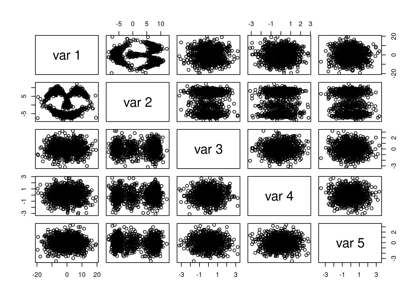 The plot demonstrates that only the first two dimensions of \(\bf x\) are far from Gaussian. The next section presents a first attempt at estimating the density using
 R and Rcpp.
An R-based and a dumb Rcpp solution
We start by creating a generic R function for kernel density estimation in R:
kdeR <- function(dker, y, x, H){
  n <- nrow(x)
  m <- nrow(y)
  out <- numeric(m)
  for(ii in 1:n){
    out <- out + dker(y, x[ii, ], H)
  }
  out <- out/n
  return(out)
}
This function works as follows:
yis the \(m \times d\) matrix at points at which we want to evaluate the k.d.e.;xis the \(n \times d\) matrix of original samples;His the bandwith matrix.
We are now ready to evaluate our k.d.e. on a grid of \(10^4\) points along the first two dimensions:
l <- 100
x1 <- seq(-20, 20, length.out = l);
x2 <- seq(-15, 15, length.out = l);
grd <- as.matrix(cbind(expand.grid(x1, x2), matrix(0, l^2, d-2)))

library(mvtnorm)
dns <- kdeR(dmvnorm, grd, x, diag(d))
Where we use the dmvnorm function from the mvtnorm package to evaluate the Gaussian kernel and we set \(\bf H\) simply to the identity matrix. We plot the k.d.e.:
library(ggplot2)
library(viridis)
## Loading required package: viridisLiteggplot(data = data.frame(x = grd[ , 1], y = grd[ , 2], z = dns),
mapping = aes(x = x, y = y, z = z, fill = z)) +
geom_raster() + geom_contour() + scale_fill_viridis_c()## Warning: The following aesthetics were dropped during statistical transformation: fill
## ℹ This can happen when ggplot fails to infer the correct grouping structure in
## the data.
## ℹ Did you forget to specify a `group` aesthetic or to convert a numerical
## variable into a factor?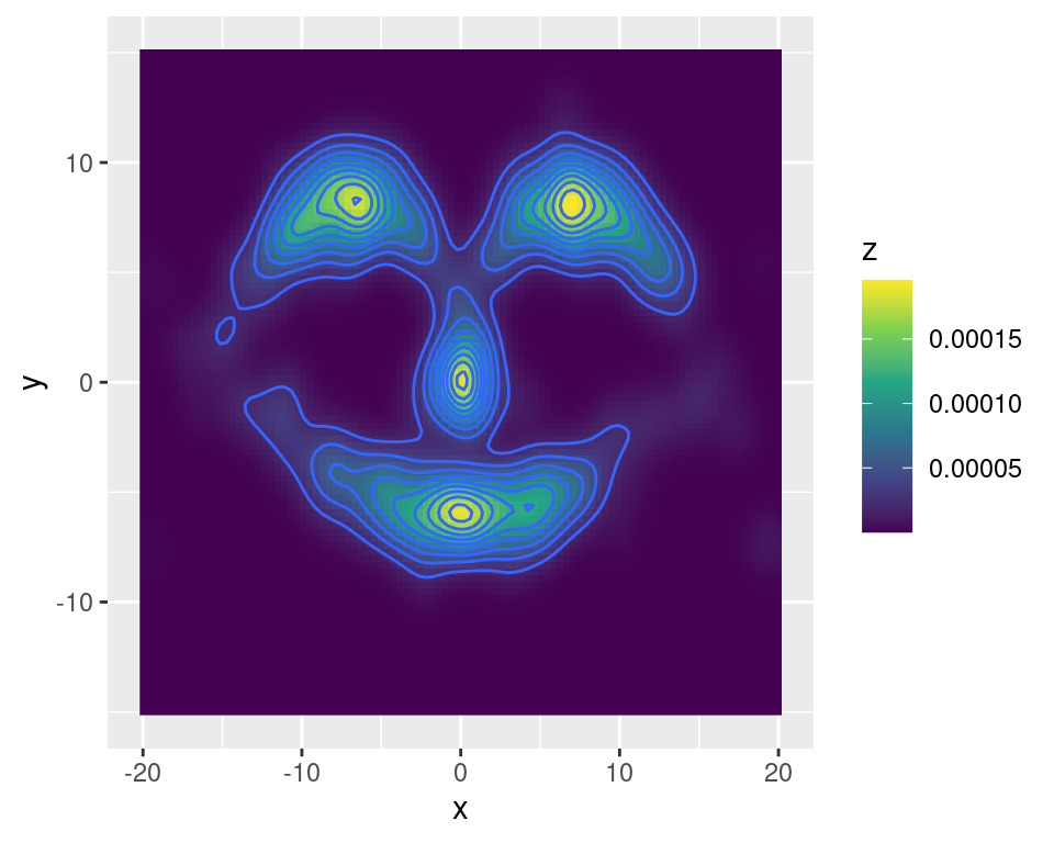
Can we speed the evaluation of the k.d.e. up using RcppArmadillo? We start with a “lazy” version, where we replace kdeR with:
library(Rcpp)
sourceCpp(code = '
// [[Rcpp::depends(RcppArmadillo)]]
#include <RcppArmadillo.h>
using namespace arma;

// [[Rcpp::export(name = "kdeLazy")]]
Rcpp::NumericVector kde_i(Rcpp::Function dker, mat& y, mat& x, mat& H) {
  unsigned int n = x.n_rows;
  unsigned int m = y.n_rows;
  vec out(m, fill::zeros);
  for(int ii = 0; ii < n; ii++){
   out += Rcpp::as<vec>(dker(y, x.row(ii), H));
  }
  out /= n;
  return Rcpp::wrap(out);
}')
Which can be used identically to kdeR and produces the same estimates:
plot(kdeR(dmvnorm, x, x, diag(d)),
kdeLazy(dmvnorm, x, x, diag(d)))
abline(0, 1, col = 2)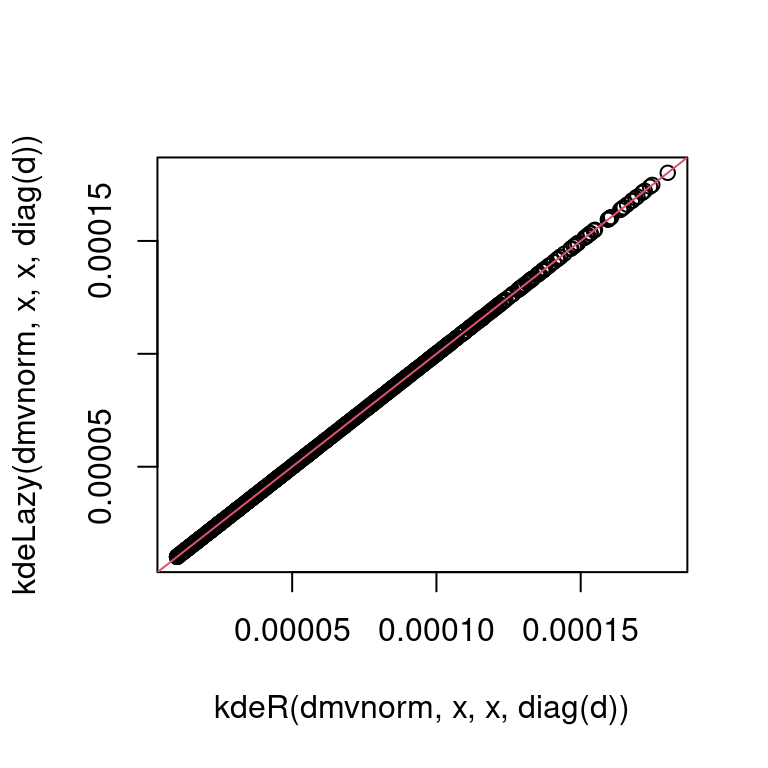 Let us compare the performance of
 kdeR and kdeLazy:
library(microbenchmark)
microbenchmark(kdeR = kdeR(dmvnorm, x, x, diag(d)),
               kdeLazy = kdeLazy(dmvnorm, x, x, diag(d)))
## Unit: milliseconds
## expr min lq mean median uq max neval
## kdeR 193.8310 197.6502 201.1110 198.8542 199.9370 277.9311 100
## kdeLazy 201.9822 206.8691 210.6367 208.8297 210.8048 289.2061 100It turns out that the Rcpp version is not faster. This demonstrates that writing part of the code in Rcpp does not automatically lead to performance gains. In particular our Rcpp code:
- calls the
dmvnRfunction to compute the Gaussian kernel. But we cannot expect anRfunction to be any faster when called fromC++rather than fromR! - the call to
Rcpp::as<vec>in the mainforloop makes a copy at each call, which is inefficient.
The next section proposes a “proper” RcppArmadillo solution for multivariate kernel density estimation.
A better RcppArmadillo solution
We start by developing an efficient RcppArmadillo function for evaluating the multivariate normal density. Before thinking about its implementation in software, we have to think about what is the most efficient way of computing it numerically. The formula for the log-density is
\[
\log \phi({\bf x}, \mu, {\bf H}) = -\frac{1}{2}({\bf x} - \mu)^T{\bf H}^{-1}({\bf x} - \mu) - \frac{d}{2} \log (2\pi) - \frac{1}{2}\log\text{det}({\bf H}).
\]
Now, for the purpose of maximizing efficiency, we have to think about how to numerically compute the quadratic form and the determinant. Let’s start with the first.
Remember that, in our k.d.e. application, \({\bf x}_1, \dots, {\bf x}_m\) are the points at which we want to evaluate the k.d.e. and \(\mu_1 = {\bf x}^o_1, \dots, \mu_n = {\bf x}^o_n\) represent the means of the kernel densities. Hence, for any fixed value of \(\mu\), we will have to evaluate the quadratic form \(m\) times. For fixed \(\mu\), we could consider two approaches:
calculate the inverse of \({\bf H}\) upfront and then calculate \(({\bf x}_i - \mu)^T{\bf H}^{-1}({\bf x}_i - \mu)\), for \(i = 1, \dots, m\);
solve the linear system \({\bf H}^{-1}({\bf x}_i - \mu) = {\bf z}_i\) and then do \(({\bf x}_i - \mu)^T{\bf z}_i\), for \(i = 1, \dots, m\);
Approach A seems quite appealing: we pay an upfront \(O(d^3)\) cost to get \({\bf H}^{-1}\) and then we pay \(O(d^2)\) cost \(m\) times to evaluate the quadratic forms. So, for \(d << m\), the dominant cost is \(O(md^2)\). Approach B seems more wasteful: solving the linear system by Gaussian elimination will cost \(O(d^3)\) operations, so doing it \(m\) times brings the dominant cost to \(O(md^3)\). However, here it is essential to take into account the fact that \(\bf H\) is positive definite, which means that approach B can be implemented much more efficiently. In particular, let \({\bf L}{\bf L}^T = {\bf H}\) be the Cholesky decomposition of \(\bf H\). Then \(({\bf x}_i - \mu)^T{\bf H}^{-1}({\bf x}_i - \mu) = ({\bf x}_i - \mu)^T({\bf L}^{-1})^T{\bf L}^{-1}({\bf x}_i - \mu)\) can be computed by:
- solving \({\bf L}^{-1}({\bf x}_i - \mu) = {\bf z}_i\) by back-substitution (recall that \(\bf L\) is lower triangular). This has cost \(O(d^2)\).
- computing \({\bf z}_i^T {\bf z}_i\) which is \(O(d)\).
Hence, the cost of approach B is \(O(m d^2)\) as well, but has the advantage of avoiding matrix inversion, which is generally less accurate than solving a linear system.
The approach we are going to follow is based on the observation that \(({\bf x}_i - \mu)^T {\bf H}^{-1}({\bf x}_i - \mu) = {\bf z}_i^T{\bf z}_i\), hence once we have obtained \({\bf z}_i\) by back-substitution as in step 1 above, we just need to calculate its squared norm at cost \(O(d)\). Having obtained the cholesky decomposition of \(\bf H\), computing its log-determinant is very cheap because \(\log\text{det}({\bf H}) = \log\text{det}({\bf L}{\bf L}^T) = 2\log\text{det}({\bf L}) = 2\log\text{trace}({\bf L})\).
Before looking at the Armadillo function to evaluate the Gaussian log-density, which we call dmvnInt, lets look at the function that will be accessed at R level:
Rcpp::NumericVector kde_i(mat& y, mat& x, mat& H) {
  unsigned int n = x.n_rows;
  unsigned int m = y.n_rows;
  vec out(m, fill::zeros);
  mat cholDec = chol(H, "lower");
  for(int ii = 0; ii < n; ii++){
   out += dmvnInt(y, x.row(ii), cholDec);
  }
  out /= n;
  return Rcpp::wrap(out);
}
This is almost identical to the function that we have used before, the main differences being the following lines:
mat cholDec = chol(H, "lower");here we are computing the Cholesky decomposition of \(\bf H\) and we are storing the lower-triangular factor incholDec;out += dmvnInt(y, x.row(ii), cholDec);evaluates a multivariate normal density, with mean vector \(\mu = {\bf x}_i^0\) and covariance \(\bf H\), at \({\bf x}_1, \dots, {\bf x}_m\). Instead of passing \(\bf H\) todmvnInt, we pass it directly its lower-triangular factor. We assume that the outputdmvnIntis anarma::vec, which can be accumulated inoutwithout callingRcpp::as<vec>.
Then, we examine the function for evaluating the multivariate Gaussian density:
vec dmvnInt(mat & X, const rowvec & mu, mat & L)
{
  unsigned int d = X.n_cols;
  unsigned int m = X.n_rows;

  vec D = L.diag();
  vec out(m);
  vec z(d);

  double acc;
  unsigned int icol, irow, ii;
  for(icol = 0; icol < m; icol++)
  {
    for(irow = 0; irow < d; irow++)
    {
     acc = 0.0;
     for(ii = 0; ii < irow; ii++) acc += z.at(ii) * L.at(irow, ii);
     z.at(irow) = ( X.at(icol, irow) - mu.at(irow) - acc ) / D.at(irow);
    }
    out.at(icol) = sum(square(z));
  }

  out = exp( - 0.5 * out - ( (d / 2.0) * log(2.0 * M_PI) + sum(log(D)) ) );

  return out;
}
the important lines are:
vec dmvnInt(mat & X, const rowvec & mu, mat & L)we return anarma::vecand all inputs are passed by reference. NOTE thatLis the lower triangular factor of the Cholesky decomposition of the covariance matrix;vec D = L.diag(); vec out(m); vec z(d);we extract the main diagonal ofL, we defined the \(m\)-dimensional vectoroutwill contain the density values at \({\bf x}_1, \dots, {\bf x}_m\) and the “working” \(d\)-dimensional vectorzwhich we will use in the main loop;for(icol = 0; icol < m; icol++)here we loop across \({\bf x}_1, \dots, {\bf x}_m\). We calculate \({\bf z}_i\) using the nested loop (next bullet point) and then we useout.at(icol) = sum(square(z));to compute and store \(||{\bf z}_i||^2\).for(irow = 0; irow < d; irow++)given \({\bf x}_i\) we get \({\bf z}_i = {\bf L}^{-1}({\bf x}_i - \mu)\) by back-substitution.
Let us now compile and load using sourceCpp:
sourceCpp(code = '
// [[Rcpp::depends(RcppArmadillo)]]
#include <RcppArmadillo.h>
using namespace arma;

vec dmvnInt(mat & X, const rowvec & mu, mat & L)
{
  unsigned int d = X.n_cols;
  unsigned int m = X.n_rows;

  vec D = L.diag();
  vec out(m);
  vec z(d);

  double acc;
  unsigned int icol, irow, ii;
  for(icol = 0; icol < m; icol++)
  {
    for(irow = 0; irow < d; irow++)
    {
     acc = 0.0;
     for(ii = 0; ii < irow; ii++) acc += z.at(ii) * L.at(irow, ii);
     z.at(irow) = ( X.at(icol, irow) - mu.at(irow) - acc ) / D.at(irow);
    }
    out.at(icol) = sum(square(z));
  }

  out = exp( - 0.5 * out - ( (d / 2.0) * log(2.0 * M_PI) + sum(log(D)) ) );

  return out;
}

// [[Rcpp::export(name = "kdeArma")]]
Rcpp::NumericVector kde_i(mat& y, mat& x, mat& H) {
  unsigned int n = x.n_rows;
  unsigned int m = y.n_rows;
  vec out(m, fill::zeros);
  mat cholDec = chol(H, "lower");
  for(int ii = 0; ii < n; ii++){
   out += dmvnInt(y, x.row(ii), cholDec);
  }
  out /= n;
  return Rcpp::wrap(out);
}')
Note that we are not exporting dmvnInt, which is used only internally by kde_i. Let’s test whether our Armadillo version works:
plot(kdeR(dmvnorm, x, x, diag(d)),
kdeArma(x, x, diag(d)))
abline(0, 1, col = 2)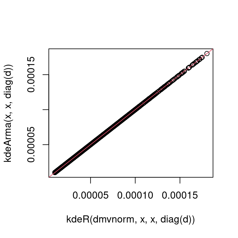 It seems so! We now compare the
 Armadillo and the R version in terms of speed:
library(microbenchmark)
microbenchmark(R = kdeR(dmvnorm, x, x, diag(d)),
               Armadillo = kdeArma(x, x, diag(d)))
## Unit: milliseconds
## expr min lq mean median uq max neval
## R 192.5236 197.5682 204.13999 201.7183 205.1449 287.2318 100
## Armadillo 34.9592 35.2923 73.21025 64.6774 108.9971 131.2905 100This is definitely better than the previous version! Note that the R version (kdeR) is not too inefficient here because, at each iteration of the main for loop, the dmvnorm function evaluates a Gaussian density at \(10^3\) data points. If we reduce the number of points at which the k.d.e. is evaluated, the performance gain increases. For instance:
library(microbenchmark)
microbenchmark(R = kdeR(dmvnorm, x[1:10, ], x, diag(d)),
               Armadillo = kdeArma(x[1:10, ], x, diag(d)))
## Unit: microseconds
## expr min lq mean median uq max neval
## R 137385.2 138358.20 140641.551 139696.60 141266.5 220721.1 100
## Armadillo 438.8 446.45 467.657 459.95 477.6 652.2 100This is attributable to a) the fact that we are computing the Cholesky decomposition of \(\bf H\) only once rather than \(n\) times, b) to the fact that for loops are much quicker in C++ that in R and c) (hopefully) that our code for computing the multivariate normal density is faster than that used by dmvtnorm.
References
Armadillo project: http://arma.sourceforge.net/
Conrad Sanderson and Ryan Curtin. Armadillo: a template-based C++ library for linear algebra. Journal of Open Source Software, Vol. 1, pp. 26, 2016.
Dirk Eddelbuettel and Conrad Sanderson, “RcppArmadillo: Accelerating R with high-performance C++ linear algebra”, Computational Statistics and Data Analysis, 2014, 71, March, pages 1054- 1063, http://dx.doi.org/10.1016/j.csda.2013.02.005. )
Fasiolo, M., de Melo, F.E. and Maskell, S., 2018. Langevin incremental mixture importance sampling. Statistics and Computing, 28(3), pp.549-561.