4. Exercise on local polynomial regression
Smoothing by local polynomial regression
Consider the following data set on solar electricity production from Sidney, Australia:
load("solarAU.RData")
head(solarAU)
## prod toy tod
## 8832 0.019 0.000000e+00 0
## 8833 0.032 5.708088e-05 1
## 8834 0.020 1.141618e-04 2
## 8835 0.038 1.712427e-04 3
## 8836 0.036 2.283235e-04 4
## 8837 0.012 2.854044e-04 5The variables are:
prodtotal production from 300 homes;toytime-of-year, going from 0 to 1 (00:00 on Jan 1st to 23:30 on 31st Dec);todtime-of-day, taking value in 0, 1, 2, …, 47 (00:00, 00:30, …, 23:30);
The interest is modelling the production as a function of the tod and toy. We will be working with log-production, which is less skewed:
solarAU$logprod <- log(solarAU$prod+0.01)We added \(0.01\) to avoid getting -Inf when the production is zero. Let’s look at the log-production as a function of the two covariates:
library(ggplot2)
library(viridis)
ggplot(solarAU,
aes(x = toy, y = tod, z = logprod)) +
stat_summary_2d() +
scale_fill_gradientn(colours = viridis(50))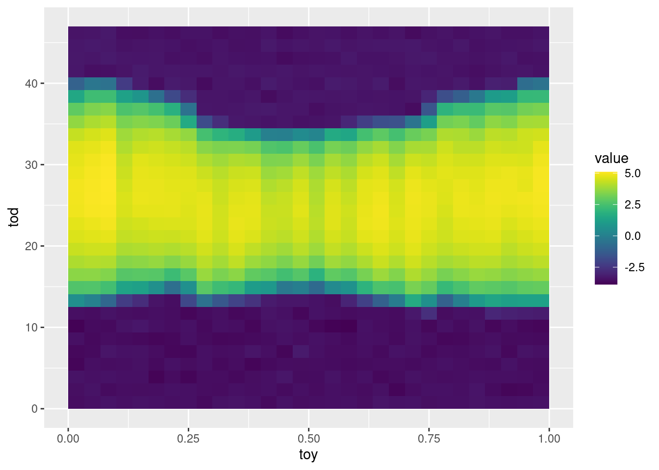 As expected, there are more hours of daylight in Austral winter, hence more production occurs during that period of the year.
Now, we aim at modelling the expected log-production, \(y\), as a function of \({\bf x} = \{\text{tod}, \text{toy}\}\). That is, we want a model for \(\mathbb{E}(y|{\bf x})\). We start with a simple polynomial regression model:
\[
\mathbb{E}(y|{\bf x}) = \beta_0 + \beta_1\text{tod} + \beta_2\text{tod}^2 + \beta_3\text{toy} + \beta_4\text{toy}^2 = \tilde{\bf x}^T\beta.
\]
where \(\tilde{\bf x} = \{\text{tod}, \text{tod}^2, \text{toy}, \text{toy}^2\}\). It is quite simple to fit this model in R:
fit <- lm(logprod ~ tod + I(tod^2) + toy + I(toy^2), data = solarAU) Q1 start Use RcppArmadillo to fit a linear regression model, that is to solve the minimization problem:
\[
\hat{\beta} = \underset{\beta}{\text{argmin}} ||{\bf y} - {\bf X}\beta||^2,
\]
where, in this example, the model matrix is given by:
X <- with(solarAU, cbind(1, tod, tod^2, toy, toy^2))Think about what numerical approach you will use (e.g., cholesky or QR decomposition) and compare the speed of your implementations with lm (of course, first you need to check whether your function gives correct results!).
Q1 end
As the following plots show, the polynomial fit is not great:
library(gridExtra)
solarAU$fitPoly <- fit$fitted.values
pl1 <- ggplot(solarAU,
aes(x = toy, y = tod, z = fitPoly)) +
stat_summary_2d() +
scale_fill_gradientn(colours = viridis(50))
pl2 <- ggplot(solarAU,
aes(x = toy, y = tod, z = logprod - fitPoly)) +
stat_summary_2d() +
scale_fill_gradientn(colours = viridis(50))
grid.arrange(pl1, pl2, ncol = 2)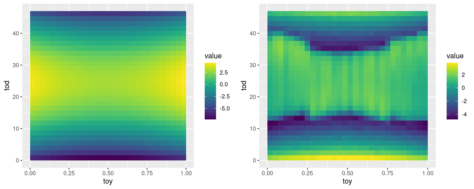 In particular, the second plot shows a clear non-linear pattern in the residuals. To improve our fit, we make our linear regression model locally adaptive by adopting a local least regression approach (see, e.g., Hastie et al, 2009, section 6.1.2 and 6.3). This consists in letting the estimated regression coefficients depend on \(\bf x\), so that \(\hat{\beta} = \hat{\beta}({\bf x})\). To achieve this, for a fixed value \({\bf x}_0\), we find \(\hat{\beta}({\bf x}_0)\) by minimizing the following objective:
\[
\hat{\beta}({\bf x}_0) = \underset{\beta}{\text{argmin}}
\sum_{i=1}^n \kappa_{\bf H}({\bf x}_0-{\bf x}_i) (y_i - \tilde{\bf x}_i^T\beta)^2,
\]
where \(\kappa_{\bf H}\) is a density kernel with positive definite bandwidth matrix \(\bf H\). Given that \(\kappa_{\bf H}({\bf x}_0-{\bf x}_i) \rightarrow 0\) as \(||{\bf x}_0-{\bf x}_i|| \rightarrow \infty\), we have that \(\hat{\beta}({\bf x}_0)\) will depend more strongly on the data points close to \({\bf x}_0\) than on those far from it.
In particular, the second plot shows a clear non-linear pattern in the residuals. To improve our fit, we make our linear regression model locally adaptive by adopting a local least regression approach (see, e.g., Hastie et al, 2009, section 6.1.2 and 6.3). This consists in letting the estimated regression coefficients depend on \(\bf x\), so that \(\hat{\beta} = \hat{\beta}({\bf x})\). To achieve this, for a fixed value \({\bf x}_0\), we find \(\hat{\beta}({\bf x}_0)\) by minimizing the following objective:
\[
\hat{\beta}({\bf x}_0) = \underset{\beta}{\text{argmin}}
\sum_{i=1}^n \kappa_{\bf H}({\bf x}_0-{\bf x}_i) (y_i - \tilde{\bf x}_i^T\beta)^2,
\]
where \(\kappa_{\bf H}\) is a density kernel with positive definite bandwidth matrix \(\bf H\). Given that \(\kappa_{\bf H}({\bf x}_0-{\bf x}_i) \rightarrow 0\) as \(||{\bf x}_0-{\bf x}_i|| \rightarrow \infty\), we have that \(\hat{\beta}({\bf x}_0)\) will depend more strongly on the data points close to \({\bf x}_0\) than on those far from it.
It is quite easy to create a function that does this in R:
library(mvtnorm)
lmLocal <- function(y, x0, X0, x, X, H){
  w <- dmvnorm(x, x0, H)
  fit <- lm(y ~ -1 + X, weights = w)
  return( t(X0) %*% coef(fit) )
}
where we are using the Gaussian kernel. Note that this requires re-estimating the model for each location \({\bf x}_0\) we are interested in. In our case:
nrow(solarAU)## [1] 17472so we need to fit the local regression model more than \(17\) thousands times to get an estimate of \(\mathbb{E}(y|{\bf x}_0)\) at each observed location. Hence, we test our local model on a sub-sample of 2000 data points:
n <- nrow(X)
nsub <- 2e3
sub <- sample(1:n, nsub, replace = FALSE)

y <- solarAU$logprod
solarAU_sub <- solarAU[sub, ]
x <- as.matrix(solarAU[c("tod", "toy")])
x0 <- x[sub, ]
X0 <- X[sub, ]
We can now obtain estimates at each subsampled location (this might take a minute or two):
predLocal <- sapply(1:nsub, function(ii){
  lmLocal(y = y, x0 = x0[ii, ], X0 = X0[ii, ], x = x, X = X, H = diag(c(1, 0.1)^2))
})
Note that we are setting \(\bf H\) to be a diagonal matrix with hand-chosen diagonal entries. Let’s look at the fit.
solarAU_sub$fitLocal <- predLocal
pl1 <- ggplot(solarAU_sub,
aes(x = toy, y = tod, z = fitLocal)) +
stat_summary_2d() +
scale_fill_gradientn(colours = viridis(50))
pl2 <- ggplot(solarAU_sub,
aes(x = toy, y = tod, z = logprod - fitLocal)) +
stat_summary_2d() +
scale_fill_gradientn(colours = viridis(50))
grid.arrange(pl1, pl2, ncol = 2)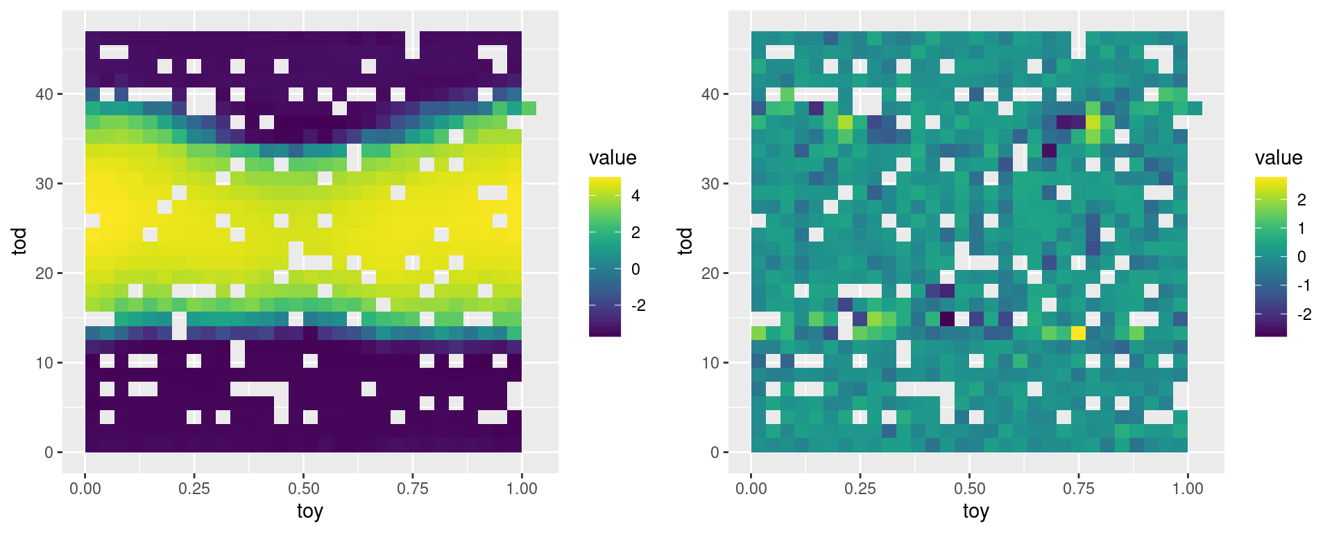 The left plot looks quite similar to the data (first plot of this document) and the residual plot shows no clear residual pattern. However, our code is very slow, so:
Q2 start To speed up the local least squares fit, implement it in RcppArmadillo and compare your solutions with the R code above in terms of speed (and correctness). If you wish, you can re-use the code we have described in a previous chapter for evaluating the multivariate normal density (but note that that function is taking as input the lower triagular factor of the Cholesky decomposition of the covariance matrix). Q2 end
Q3 start Above, we have chosen the bandwidth matrix \(\bf H\) manually. Once you have created an RcppArmadillo function for local linear regression, set up a cross-validation routine for tuning the bandwidth matrix automatically. Q3 end
References
- Hastie, T., Tibshirani, R. and Friedman, J., 2009. The elements of statistical learning: data mining, inference, and prediction (Second Edition). Springer.