Smoothing by local polynomial regression

Here we consider an Irish smart meter data set which can be found in the electBook package. At the time of writing electBook is available only on Github, hence we need to install it from there using devtools:

# Install electBook only if it is not already installed
if( !require(electBook) ){
  library(devtools)
  install_github("mfasiolo/electBook")
  library(electBook)
}

We can now load the data:

library(electBook)
data(Irish)

See ?Irish or [https://awllee.github.io/sc1/tidyverse/data_reshaping_tidyr/] for details about the data. Let us concatenate the electricity demand from all households into a single vector:

y <- do.call("c", Irish$indCons)
y <- y - mean(y)
str(y)
# Named num [1:44886928] -0.477 -0.366 -0.405 -0.476 -0.366 ...
# - attr(*, "names")= chr [1:44886928] "I10021" "I10022" "I10023" "I10024" ...

We have over 44 million observations, here we plot as sub-set:

ncust <- ncol(Irish$indCons) 

x <- rep(Irish$extra$tod, ncust)

n <- length(x)
ss <- sample(1:n, 1e4)
plot(x[ss], y[ss], col = "grey")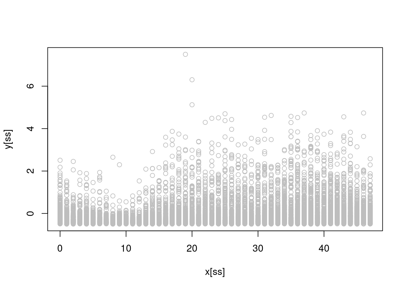

where the \(x\)-axis here represents the time of day (0 is midnight and 47 is 23:30).

We want to model the relation between the time of day (x) and the demand (y). We start with a simple univariate regression model \(\mathbb{E}(y|x) = \beta_1 x\) (note that we do not need an intercept as we have centered y above). Here is a simple function to fit the model by least squares:

reg1D <- function(y, x){
  
  b <- t(x) %*% y / (t(x) %*% x)  
  
  return(b)
  
}

Let’s compare this with the standard lm() function:

system.time( lm(y ~ -1 + x)$coeff )[3]
11.518 

system.time( reg1D(y, x) )[3]
0.92

Note that lm is much slower (probably because it computes many quantities that our function does not compute).

Q1 start Implement a parallel version of reg1D using RcppParallel. You might want use OpenMP and/or some of the functions provided by RcppParallel (e.g., parallelReduce) to parallelise you code. Make sure that you use thread-safe data structures. Compare your function to reg1D in terms of exactness and timing. Q1 end

Looking at the scatterplot above, it is clear that the linear model will provide a poor fit, in fact:

ss <- sort( sample(1:n, 1e4) )
plot(x[ss], y[ss], col = "grey")
abline(a = 0, b = reg1D(y, x), col = 2, lwd = 2)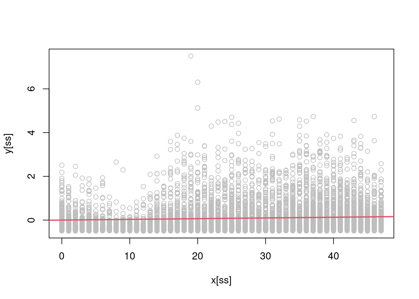

is arguably a pretty poor fit! Let’s try to do better by fitting a polynomial regression such as \(\mathbb{E}(y|x) = \beta_0 + \beta_1 x + \beta_2 x^2 + \beta_3 x^3\) (note that we have included an intercept here, despite \(y\) being centered. The reason will become clear later on). A multivariate linear regression model, with model matrix X, can be fitted using the following function:

regMD <- function(y, X){
  
  XtX <- t(X) %*% X
  
  C <- chol(XtX)
  
  b <- backsolve(C, forwardsolve(t(C), t(X) %*% y) )
  
  return(b)
  
}

This function calculates the cholesky decomposition \(\bf C^T \bf C = \bf X^T \bf X\) where \(\bf C\) is upper triangular. Then \(\hat{\bf \beta} = \bf C^{-1}\bf C^{-T}\bf X^T\bf y\), which is solved by computing \(\bf z = \bf C^{-T}\bf X^T\bf y\) by forward-solving the lower-triangular system and then \(\hat{\bf \beta} = \bf C^{-1} \bf z\) by back-solving the upper-triangular system. Let’s see whether our function works:

X <- cbind(1, x, x^2, x^3)

b <- regMD(y, X)

b_lm <- lm(y ~ -1 + X)$coeff

Xu <- cbind(1, 0:47, (0:47)^2, (0:47)^3)
plot(x[ss], y[ss], col = "grey")
lines(0:47, Xu %*% b, col = 2, lwd = 3)
lines(0:47, Xu %*% b_lm, col = 1, lty = 2)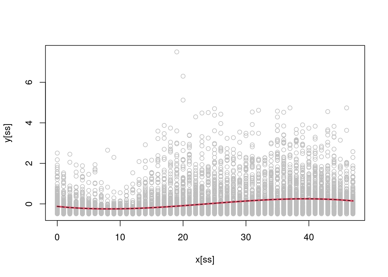

As one would hope, our solution coincides with the one provided by lm().

Q2 start Implement a parallel version of regMD using RcppParallel and compare your function to regMD in terms of exactness and timing. Q2 end

The polynomial fit is better but we can do even better using local polynomial regression. This is a function for basic one dimensional local polynomial regression (using a Gaussian kernel):

regMD_local <- function(y, X, x0, x, h){
  
  w <- dnorm(x0, x, h)
  w <- w / sum(x) * length(y)
  
  wY <- y * sqrt(w)
  wX <- X * sqrt(w)
  wXtwX <- t(wX) %*% wX
  
  C <- chol(wXtwX)
  
  b <- backsolve(C, forwardsolve(t(C), t(wX) %*% wY) )
  
  return(b)
  
}

As always, it is work checking whether our function works by comparing it with lm():

b <- regMD_local(y, X, x0 = 35, x = x, h = 5)
b_lm <- lm(y ~ -1 + X, weights = dnorm(35, x, 5))$coeff

plot(x[ss], y[ss], col = "grey")
lines(0:47, Xu %*% b, col = 2, lwd = 3)
lines(0:47, Xu %*% b_lm, col = 1, lty = 2)
abline(v = 35, lty = 2)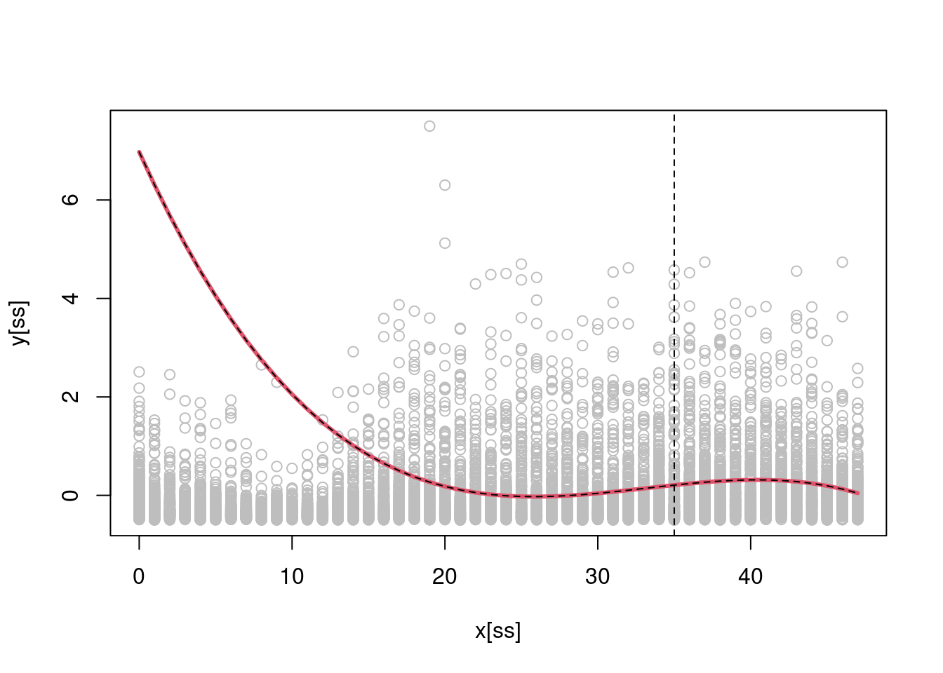

It seems so. To evaluate our fitted function at several points on the \(x\)-axis, we do (NOTE this takes a few minutes to run):

f <- lapply(0:47, function(.x ) regMD_local(y, X, x0 = .x, x = x, h = 5))

plot(x[ss], y[ss], col = "grey")
lines(0:47, sapply(1:48, function(ii) Xu[ii, ] %*% f[[ii]]), col = 2, lwd = 3, type = 'b')

Q3 start Implement a parallel version of regMD_local using RcppParallel and compare your function to regMD_local in terms of exactness and timing. Q3 end

Q4 start Consider these lines of code:

  w <- dnorm(x0, x, h)
  w <- w / sum(x)

In principle the weights should sum to one, but for example:

x <- c(100, 200, 300)
( w <- dnorm(0, x, 1) )

## [1] 0 0 0

( w <- w / sum(x) ) 

## [1] 0 0 0

as you can see, all the weight are 0! The numerically stable way of computing this is:

lw <- dnorm(0, x, 1, log = TRUE)
mlw <- max(lw)
( w <- exp(lw - mlw) / sum(exp(lw - mlw)) ) 

## [1] 1 0 0

Think about why this solution is preferable and implement a parallel version of it. Q4 end

Q5 start Assume that new data becomes available, that is the model matrix is updated to \(\bf X \leftarrow [\bf X_{\text{old}}^T, \bf X_{\text{new}}^T]^T\) (new rows of data have been added). Assuming that you have stored \(\bf X_{\text{old}}^T \bf W_{\text{old}} \bf X_{\text{old}}\), how would you efficiently update your fit? Q5 end