Some diagnostics for a fitted gam model

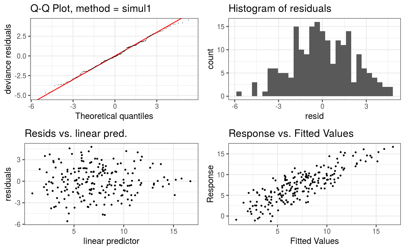
Takes a fitted GAM model and produces some diagnostic information about the fitting procedure and results. The default is to produce 4 residual plots, some information about the convergence of the smoothness selection optimization, and to run diagnostic tests of whether the basis dimension choises are adequate.

# S3 method for gamViz
check(
  obj,
  type = c("auto", "deviance", "pearson", "response", "tunif", "tnormal"),
  k.sample = 5000,
  k.rep = 200,
  maxpo = 10000,
  a.qq = list(),
  a.hist = list(),
  a.respoi = list(),
  ...
)

Arguments

obj	an object of class gamViz, the output of a getViz() call.
type	type of residuals, see residuals.gamViz, used in all plots.
k.sample	above this k testing uses a random sub-sample of data.
k.rep	how many re-shuffles to do to get p-value for k testing.
maxpo	maximum number of residuals points that will be plotted in the scatter-plots. If number of datapoints > maxpo, then a subsample of maxpo points will be plotted.
a.qq	list of arguments to be passed to qq.gamViz. See qq.gamViz.
a.hist	list of arguments to be passed to ggplot2::geom_histogram.
a.respoi	list of arguments to be passed to ggplot2::geom_point.
...	currently not used.

Value

An object of class checkGam, which is simply a list of ggplot objects.

Details

This is a essentially a re-write of mgcv::gam.check using ggplot2. See mgcv::gam.check for details.

Examples

library(mgcViz)
set.seed(0)
dat <- gamSim(1, n = 200)
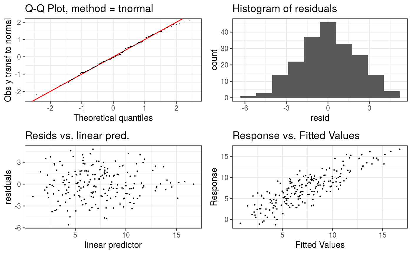
#> Gu & Wahba 4 term additive model
b <- gam(y ~ s(x0) + s(x1) + s(x2) + s(x3), data = dat)
b <- getViz(b)

# Checks using default options
check(b)
#> 
#> Method: GCV   Optimizer: magic
#> Smoothing parameter selection converged after 8 iterations.
#> The RMS GCV score gradient at convergence was 1.072609e-05 .
#> The Hessian was positive definite.
#> Model rank =  37 / 37 
#> 
#> Basis dimension (k) checking results. Low p-value (k-index<1) may
#> indicate that k is too low, especially if edf is close to k'.
#> 
#>         k'  edf k-index p-value
#> s(x0) 9.00 2.32    1.00    0.51
#> s(x1) 9.00 2.31    0.97    0.30
#> s(x2) 9.00 7.65    0.96    0.27
#> s(x3) 9.00 1.23    1.04    0.67
#> `stat_bin()` using `bins = 30`. Pick better value with `binwidth`.

# Change some algorithmic and graphical parameters
check(b,
      a.qq = list(method = "tnorm",
                  a.cipoly = list(fill = "light blue")),
      a.respoi = list(size = 0.2),
      a.hist = list(bins = 10))
#> 
#> Method: GCV   Optimizer: magic
#> Smoothing parameter selection converged after 8 iterations.
#> The RMS GCV score gradient at convergence was 1.072609e-05 .
#> The Hessian was positive definite.
#> Model rank =  37 / 37 
#> 
#> Basis dimension (k) checking results. Low p-value (k-index<1) may
#> indicate that k is too low, especially if edf is close to k'.
#> 
#>         k'  edf k-index p-value
#> s(x0) 9.00 2.32    1.00    0.45
#> s(x1) 9.00 2.31    0.97    0.33
#> s(x2) 9.00 7.65    0.96    0.24
#> s(x3) 9.00 1.23    1.04    0.68