Checking GAM residuals along two covariates

This function extracts the residuals of a fitted GAM model, and plots them according to the values of two covariates. Then several visual residuals diagnostics can be plotted by adding layers.

check2D(
  o,
  x1,
  x2,
  type = "auto",
  maxpo = 10000,
  na.rm = TRUE,
  trans = NULL,
  useSim = TRUE
)

Arguments

o	an object of class gamViz.
x1	it can be either a) a single character, b) a numeric vector or c) a list of characters. In case a) it should be the name of one of the variables in the dataframe used to fit o. In case b) its length should be equal to the length of o$y. In case c) it should be a list of names of variables in the dataframe used to fit o.
x2	same as x2, but this will appear on the y-axis.
type	the type of residuals to be used. See residuals.gamViz. If "type == y" then the raw observations will be used.
maxpo	maximum number of residuals points that will be used by layers such as l_rug(). If number of datapoints > maxpo, then a subsample of maxpo points will be taken.
na.rm	if TRUE missing cases in x or y will be dropped out
trans	function used to transform the observed and simulated residuals or responses. It must take a vector of as input, and must return a vector of the same length.
useSim	if FALSE then the simulated responses contained in object o will not be used by this function or by any of the layers that can be used with its output.

Value

The function will return an object of class c("plotSmooth", "gg"), unless arguments x1 and/or x2 are lists. If they are lists of the same length, then the function will return an object of class c("plotGam", "gg") containing a checking plot for each pair of variables. If x1 is a list and x2 is not specified, the function will return an object of class c("plotGam", "gg") containing a plot for each unique combination of the variables in x1.

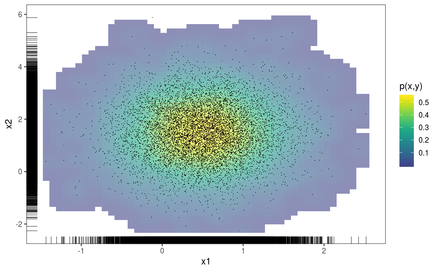
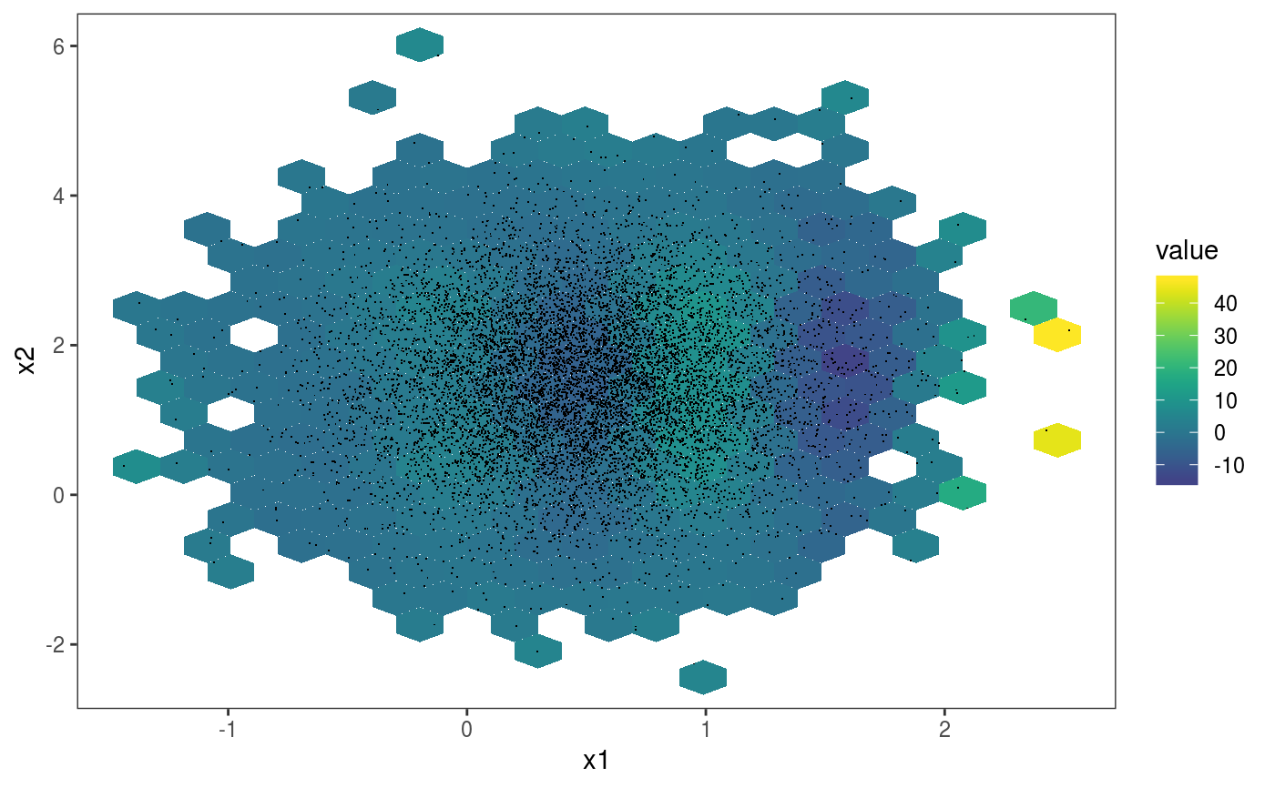
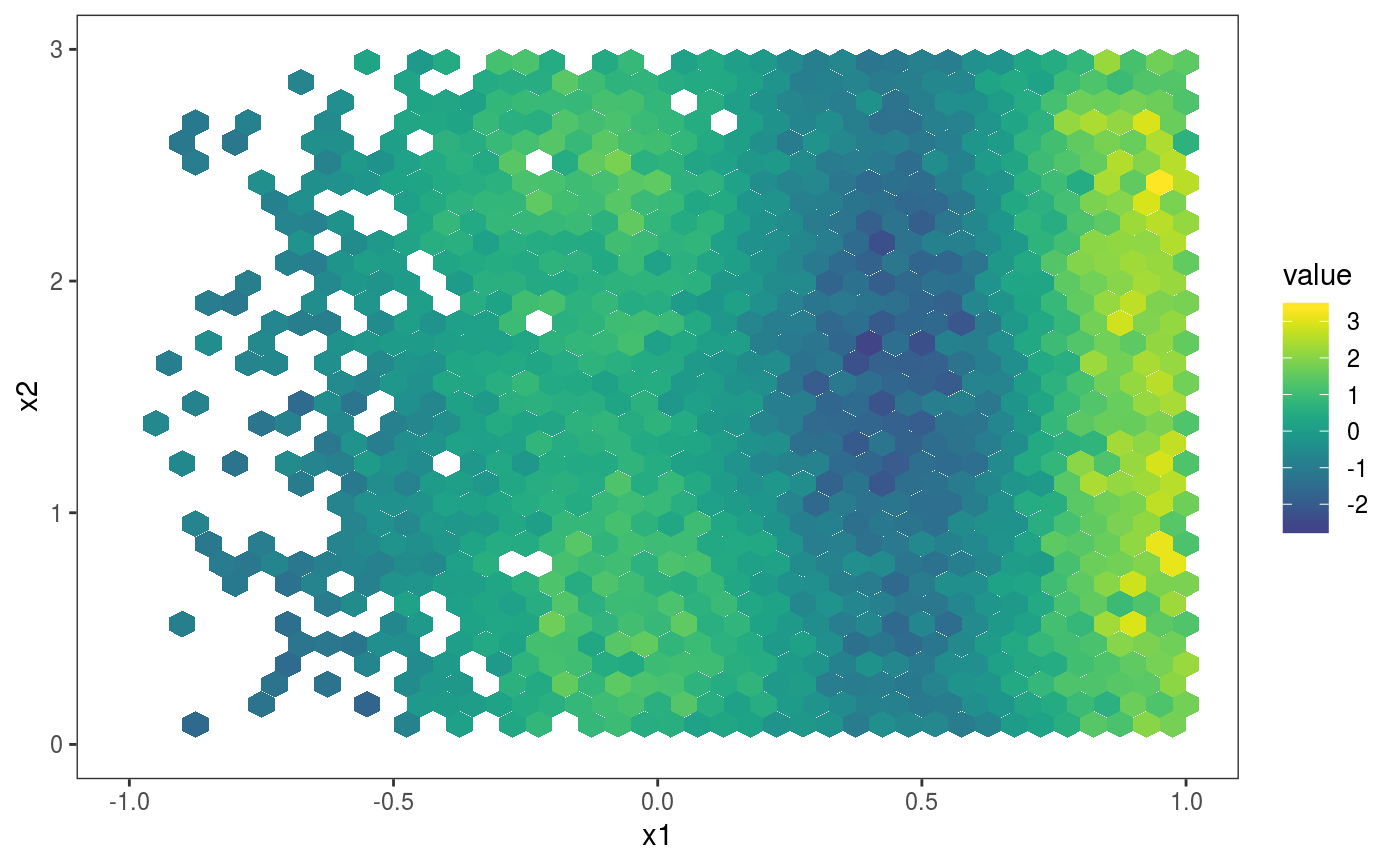
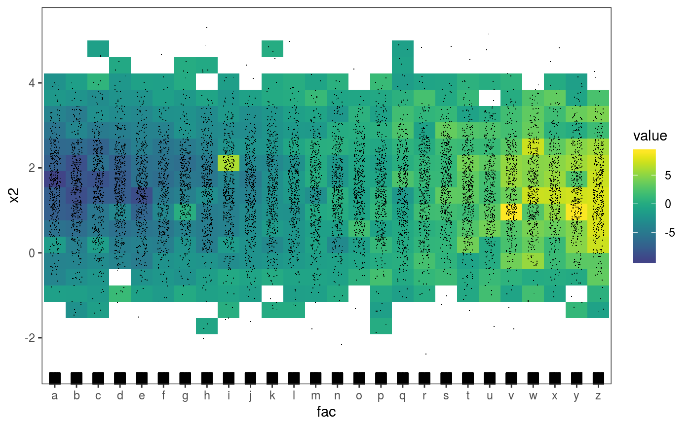
Examples

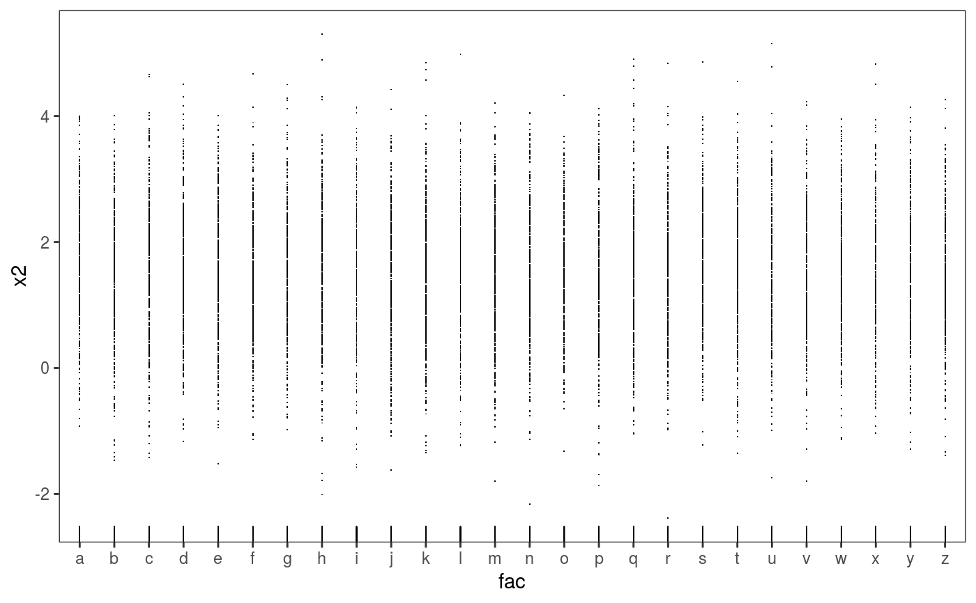
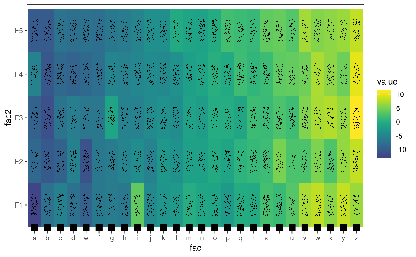
library(mgcViz);
#### Example 1: Rosenbrock function
# Simulate data
n <- 1e4
X <- data.frame("x1"=rnorm(n, 0.5, 0.5), "x2"=rnorm(n, 1.5, 1))
X$y <- (1-X$x1)^2 + 100*(X$x2 - X$x1^2)^2 + rnorm(n, 0, 2)
b <- bam(y ~ te(x1, x2, k = 5), data = X, discrete = TRUE)
b <- getViz(b, nsim = 50)

# Plot joint density of observed covariate x1 and x2
check2D(b, x1 = "x1", x2 = "x2") + l_rug() + l_dens(type="joint", alpha=0.6) + l_points()

# Look at how mean of residuals varies across x1 and x2
check2D(b, x1 = "x1", x2 = "x2") + l_gridCheck2D() + l_points()

# Can't see much in previous plot, let's zoom in central area, where most
# data is. Here we can clearly see that the mean model is mispecified
check2D(b, x1 = "x1", x2 = "x2") + l_gridCheck2D(bw = c(0.05, 0.1)) +
                                   xlim(-1, 1) + ylim(0, 3)
# Fit can be improved by increasing k in the bam() call

#### Example 2: checking along factor variables
# Simulate data where variance changes along factor variable "fac"
n <- 1e4
X <- data.frame("x1"=rnorm(n, 0.5, 0.5), "x2"=rnorm(n, 1.5, 1))
X$fac <- as.factor( sample(letters, n, replace = TRUE) )
X$fac2 <- as.factor( sample(c("F1", "F2", "F3", "F4", "F5"), n, replace = TRUE) )
X$y <- (1-X$x1)^2 + 5*(X$x2 - X$x1^2)^2 + 0.1*as.numeric(X$fac) * rnorm(n, 0, 2)
b <- bam(y ~ te(x1, x2, k = 5) + fac + fac2, data = X, discrete = TRUE)
b <- getViz(b, nsim = 50)

# Check standard deviation of residuals along covariates "x1" and "fac"
a <- check2D(b, x1 = "x2", x2 = "fac")
#> check2D likes to have factor variables on x axis: I am swapping the coordinates.
a + l_gridCheck2D(gridFun = sd) + l_rug() + l_points()

# Points and rug are jittered by default, but we can over-ride this
a + l_rug(position = position_jitter(width = 0, height = 0)) +
  l_points(position = position_jitter(width = 0, height = 0))

# Check standard deviation of residuals along the two factor variables
a <- check2D(b, x1 = "fac", x2 = "fac2")
a + l_gridCheck2D(gridFun = sd, bw = c(1, 4)) + l_rug() + l_points()
#> Warning: no non-missing arguments to min; returning Inf
#> Warning: no non-missing arguments to max; returning -Inf