Binning and checking GAM residuals

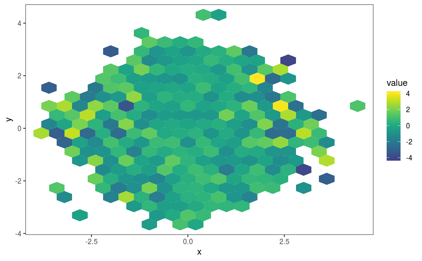
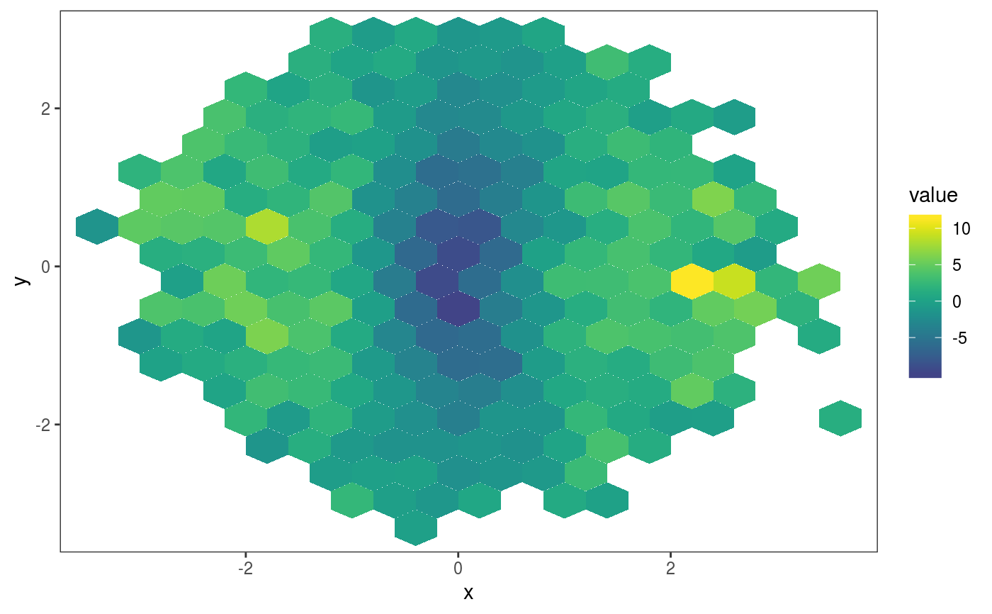
This layer bins the residuals, r, according to the value of the corresponding covariates, x1 and x2. Then the residuals in each bin are summarized using a scalar-valued statistic. Confidence intervals for the statistic corresponding to each bin can be obtained by simulating residuals from the fitted GAM model, which are then binned and summarized. Mainly useful in conjuction with check2D.

l_gridCheck2D(gridFun = mean, bw = c(NA, NA), stand = TRUE, binFun = NULL, ...)

Arguments

gridFun	scalar-valued function used to summarize the residuals in each bin.
bw	numeric vector giving bin width in the vertical and horizontal directions. See the binwidth arguments in ?ggplot2::stat_summary_hex. If left to NA, it will be set to 1/20 of the ranges of x1 and x2.
stand	if left to TRUE then the observed statistic in the i-th cell is normalized using the simulated statistics in that same cell. That is, we will actually plot std_stat = (obs_stat-mean(sim_stat))/sd(sim_stat).
binFun	the ggplot2 function used to perform the binning. By default it is either ggplot2::stat_summary_2d or ggplot2::stat_summary_hex, depending on the class of the covariates x1 and x2.
...	graphical arguments to be passed to ggplot2::stat_summary_hex.

Value

An object of class gamLayer

Examples

library(mgcViz);
set.seed(4124)
n <- 1e4
x <- rnorm(n); y <- rnorm(n);

# Residuals are heteroscedastic w.r.t. x
ob <- (x)^2 + (y)^2 + (1*abs(x) + 1)  * rnorm(n)
b <- bam(ob ~ s(x,k=30) + s(y, k=30), discrete = TRUE)
b <- getViz(b, nsim = 50)

# Don't see much by looking at mean
check2D(b, "x", "y") + l_gridCheck2D(gridFun = mean, bw = c(0.4, 0.4))

# Variance pattern along x-axis clearer now
check2D(b, "x", "y") + l_gridCheck2D(gridFun = sd, bw = c(0.4, 0.4))