Fit a GAMM or GAMM4 model and get a gamViz object

These are wrappers that fit GAM models using mgcv::gamm or gamm4::gamm4 and convert them to a gamViz object using the getViz function. It is essentially a shortcut.

gamm4V(
  formula,
  random,
  family = gaussian(),
  data = list(),
  REML = TRUE,
  aGam = list(),
  aViz = list(),
  keepGAMObj = FALSE
)

gammV(
  formula,
  random,
  family = gaussian(),
  data = list(),
  method = "REML",
  aGam = list(),
  aViz = list(),
  keepGAMObj = FALSE
)

Arguments

formula, random, family, data	same arguments as in mgcv::gamm or gamm4::gamm4.
REML	same as in gamm4::gamm4
aGam	list of further arguments to be passed to mgcv::gamm or gamm4::gamm4.
aViz	list of arguments to be passed to getViz.
keepGAMObj	if TRUE a copy of the gamViz Object is kept under $gam to assure compatibility with mgcv::gamm and gamm4::gamm4. Defaults to FALSE.
method	same as in mgcv::gamm

Value

An object of class "gamViz" which can, for instance, be plotted using plot.gamViz. Also the object has the following additional elements:

• lme mixed model as in mgcv::gamm

• mer mixed model as in gamm4::gamm4

• gam a copy of the gamViz Object if setting keepGAMObj = TRUE.

Details

WARNING: Model comparisons (e.g. with anova) should only be done using the mixed model part as described in gamm4::gamm4. For mgcv::gamm please refer to the original help file.

Examples

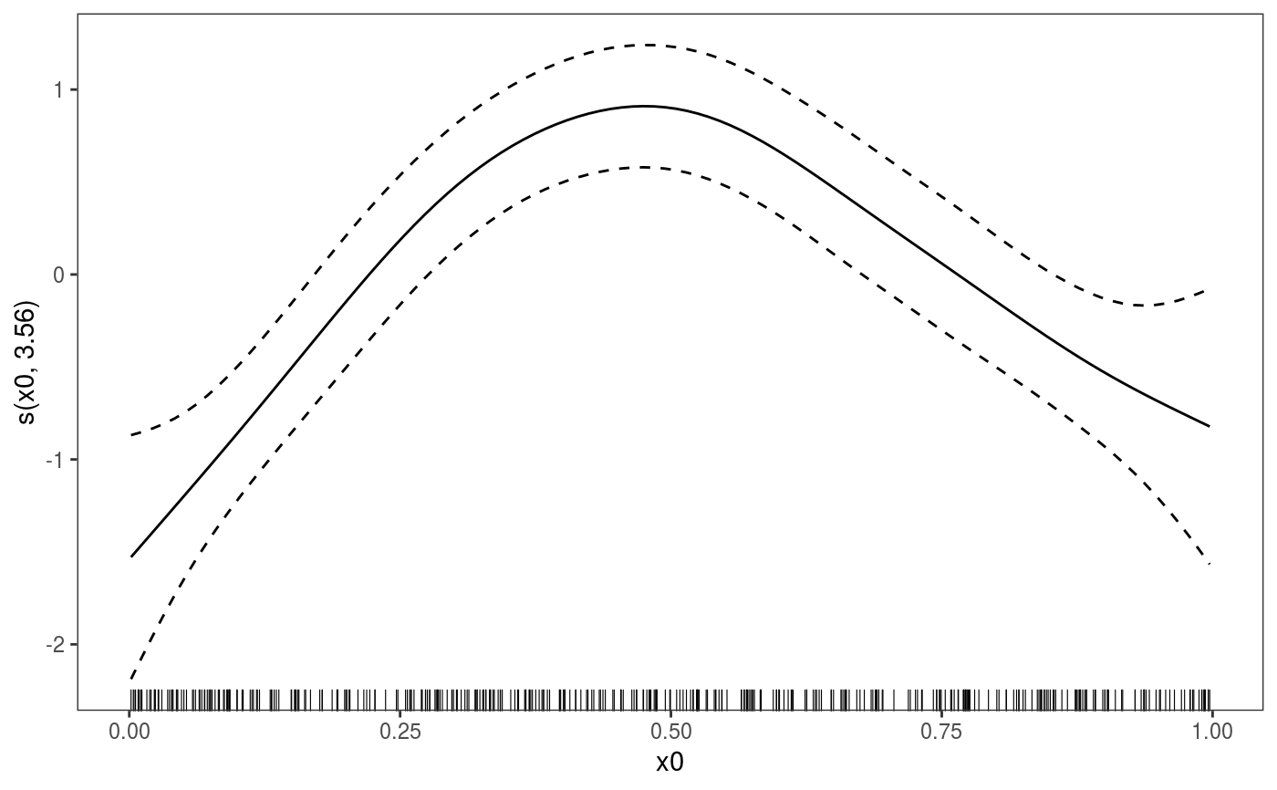
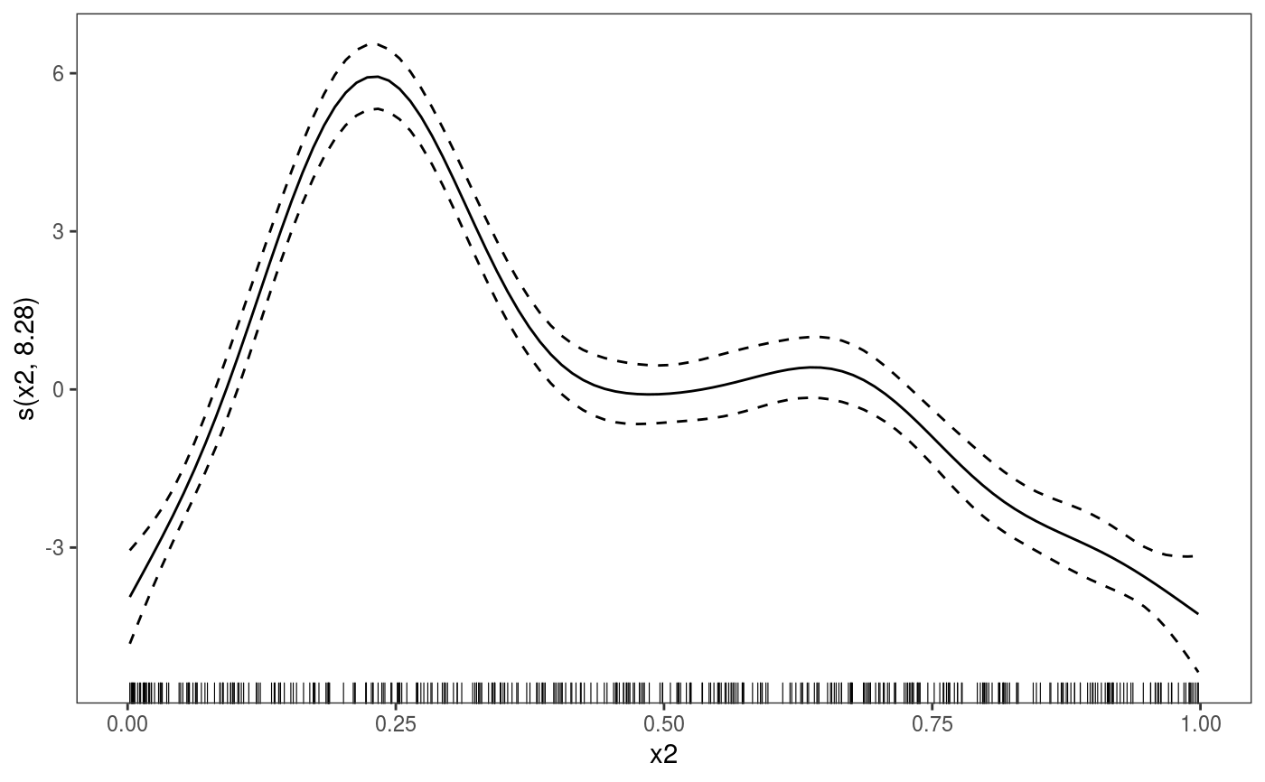
##### gam example
library(mgcViz)
# Simulate data
dat <- gamSim(1,n=400,scale=2) ## simulate 4 term additive truth
#> Gu & Wahba 4 term additive model
## Now add 20 level random effect `fac'...
dat$fac <- fac <- as.factor(sample(1:20,400,replace=TRUE))
dat$y <- dat$y + model.matrix(~fac-1) %*% rnorm(20) * 0.5

br <- gammV(y~s(x0)+x1+s(x2), data=dat,random=list(fac=~1))
summary(br)
#> 
#> Family: gaussian 
#> Link function: identity 
#> 
#> Formula:
#> y ~ s(x0) + x1 + s(x2)
#> 
#> Parametric coefficients:
#>             Estimate Std. Error t value Pr(>|t|)    
#> (Intercept)   4.4441     0.2391   18.58   <2e-16 ***
#> x1            6.3160     0.3658   17.27   <2e-16 ***
#> ---
#> Signif. codes:  0 ‘***’ 0.001 ‘**’ 0.01 ‘*’ 0.05 ‘.’ 0.1 ‘ ’ 1
#> 
#> Approximate significance of smooth terms:
#>         edf Ref.df     F  p-value    
#> s(x0) 3.561  3.561 13.59 3.63e-09 ***
#> s(x2) 8.277  8.277 78.83  < 2e-16 ***
#> ---
#> Signif. codes:  0 ‘***’ 0.001 ‘**’ 0.01 ‘*’ 0.05 ‘.’ 0.1 ‘ ’ 1
#> 
#> R-sq.(adj) =  0.711   
#>   Scale est. = 4.3612    n = 400
plot(br)
#> Hit <Return> to see next plot:
#> Hit <Return> to see next plot:

summary(br$lme)
#> Linear mixed-effects model fit by REML
#>  Data: strip.offset(mf) 
#>        AIC      BIC    logLik
#>   1794.035 1825.886 -889.0176
#> 
#> Random effects:
#>  Formula: ~Xr - 1 | g
#>  Structure: pdIdnot
#>              Xr1      Xr2      Xr3      Xr4      Xr5      Xr6      Xr7      Xr8
#> StdDev: 2.277582 2.277582 2.277582 2.277582 2.277582 2.277582 2.277582 2.277582
#> 
#>  Formula: ~Xr.0 - 1 | g.0 %in% g
#>  Structure: pdIdnot
#>            Xr.01    Xr.02    Xr.03    Xr.04    Xr.05    Xr.06    Xr.07    Xr.08
#> StdDev: 22.89384 22.89384 22.89384 22.89384 22.89384 22.89384 22.89384 22.89384
#> 
#>  Formula: ~1 | fac %in% g.0 %in% g
#>         (Intercept) Residual
#> StdDev:   0.5101666 2.088341
#> 
#> Fixed effects: y.0 ~ X - 1 
#>                 Value Std.Error  DF   t-value p-value
#> X(Intercept) 4.444137 0.2391326 377 18.584404  0.0000
#> Xx1          6.316044 0.3658366 377 17.264660  0.0000
#> Xs(x0)Fx1    0.579127 0.7092469 377  0.816538  0.4147
#> Xs(x2)Fx1    3.409999 2.0166404 377  1.690931  0.0917
#>  Correlation: 
#>           X(Int) Xx1    X(0)F1
#> Xx1       -0.759              
#> Xs(x0)Fx1 -0.006  0.005       
#> Xs(x2)Fx1  0.038 -0.050 -0.021
#> 
#> Standardized Within-Group Residuals:
#>          Min           Q1          Med           Q3          Max 
#> -3.526741115 -0.601897375 -0.001453839  0.676182616  3.304378003 
#> 
#> Number of Observations: 400
#> Number of Groups: 
#>                   g          g.0 %in% g fac %in% g.0 %in% g 
#>                   1                   1                  20 

if (FALSE) {
## gamm4::gamm4 example
br4 <- gamm4V(y~s(x0)+x1+s(x2),data=dat,random=~(1|fac))
summary(br4)
plot(br4)

summary(br4$mer)
}