Basic GAM plotting

This function is the mgcViz equivalent of plot.gam. It is the workhorse of the mgcViz package, and allows plotting (almost) any type of smooth, parametric or random effects. It is basically a wrapper around plotting methods that are specific to individual smooth effect classes (such as plot.mgcv.smooth.1D and plot.random.effect).

# S3 method for gamViz
plot(x, n = 100, n2 = 40, select = NULL, allTerms = FALSE, ...)

Arguments

x	an object of class gamViz, the output of a getViz call.
n	number of points used for each 1-d plot. For a nice smooth plot this needs to be several times the estimated degrees of freedom for the smooth.
n2	square root of number of grid points used for plotting 2D functions effects using contours or heatmaps.
select	allows plotting a subset of model terms. For instance, if you just want the plot for the second smooth term, set select = 2. Parametric effects always come after smooth or random effects.
allTerms	if TRUE also the parametric effects will be plotted.
...	other parameters, such as maxpo or trans, to be passed to the specific plotting methods for each effect (e.g. to plot.mgcv.smooth.1D).

Value

An object of class c("plotGam", "gg").

Examples

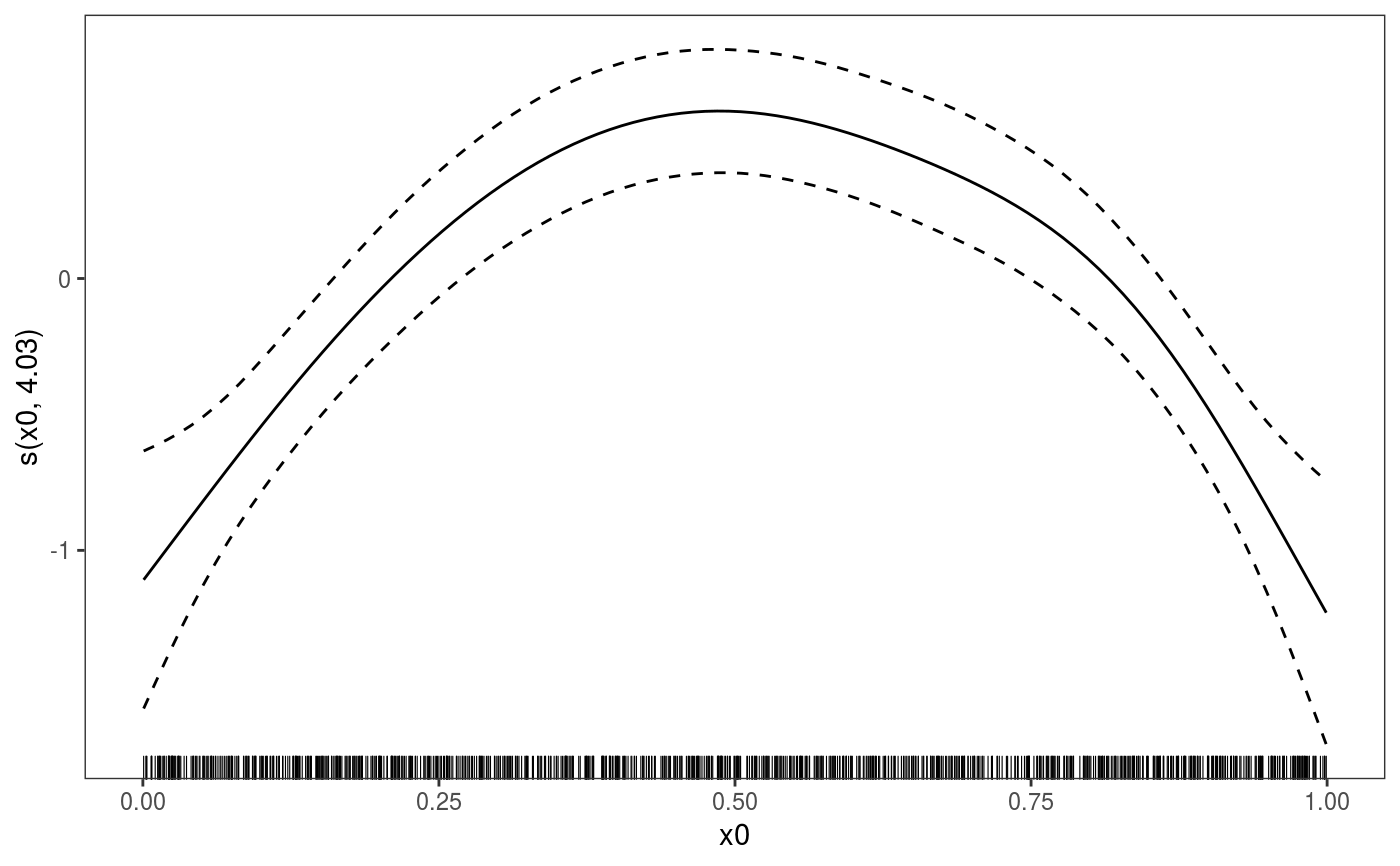
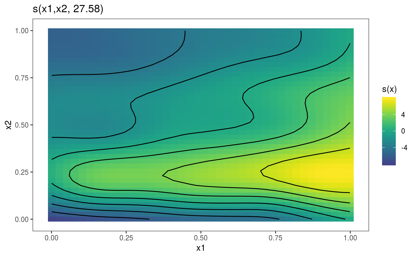
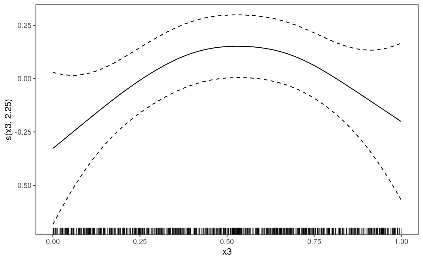
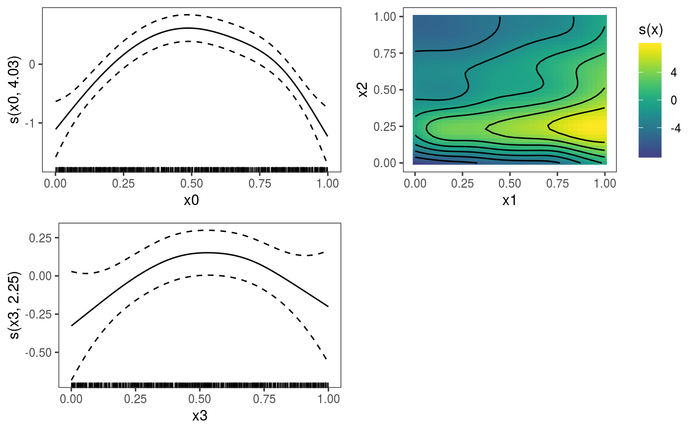
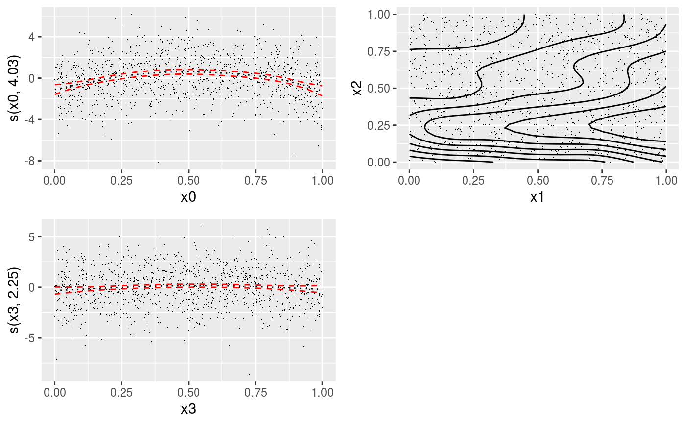
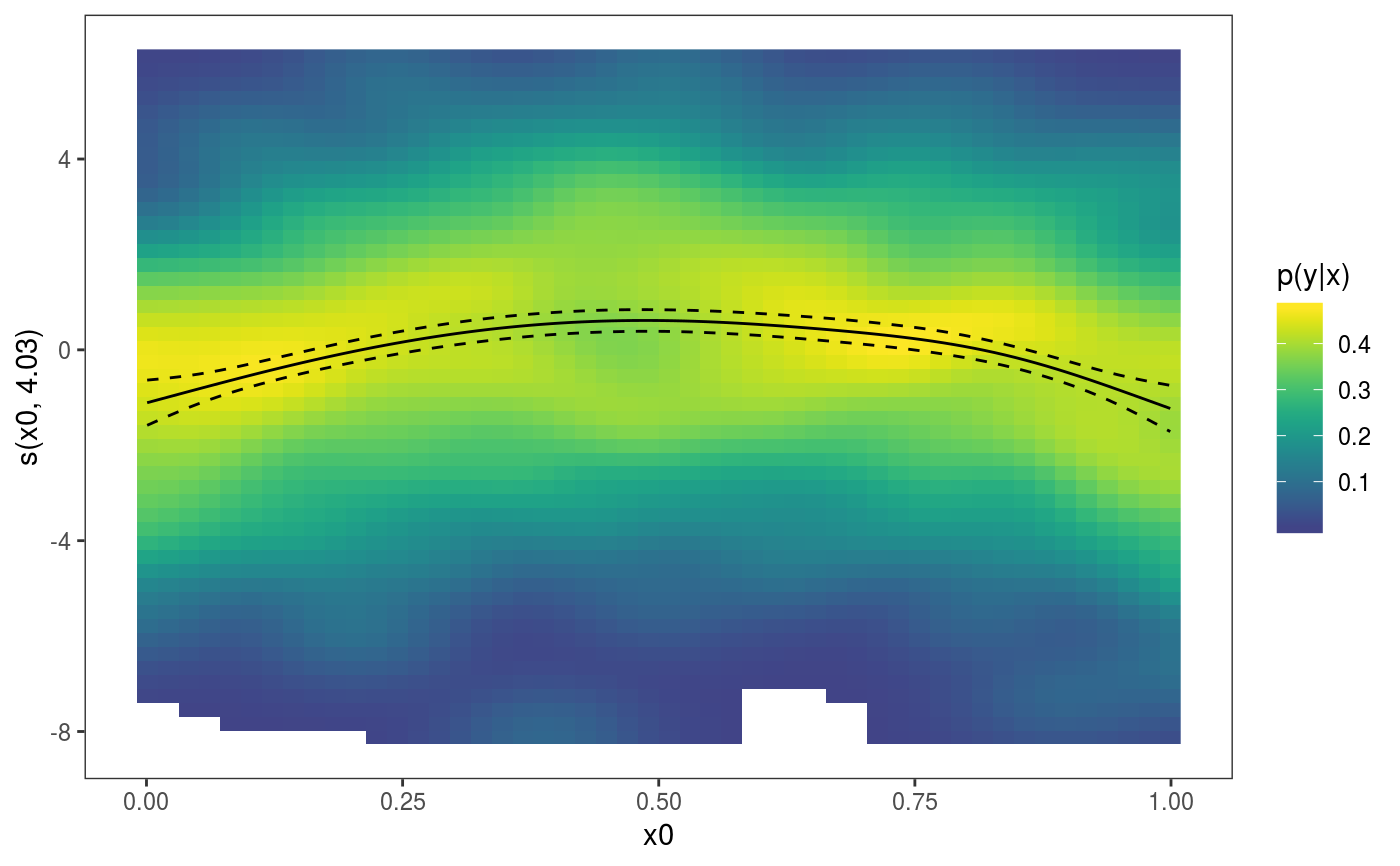
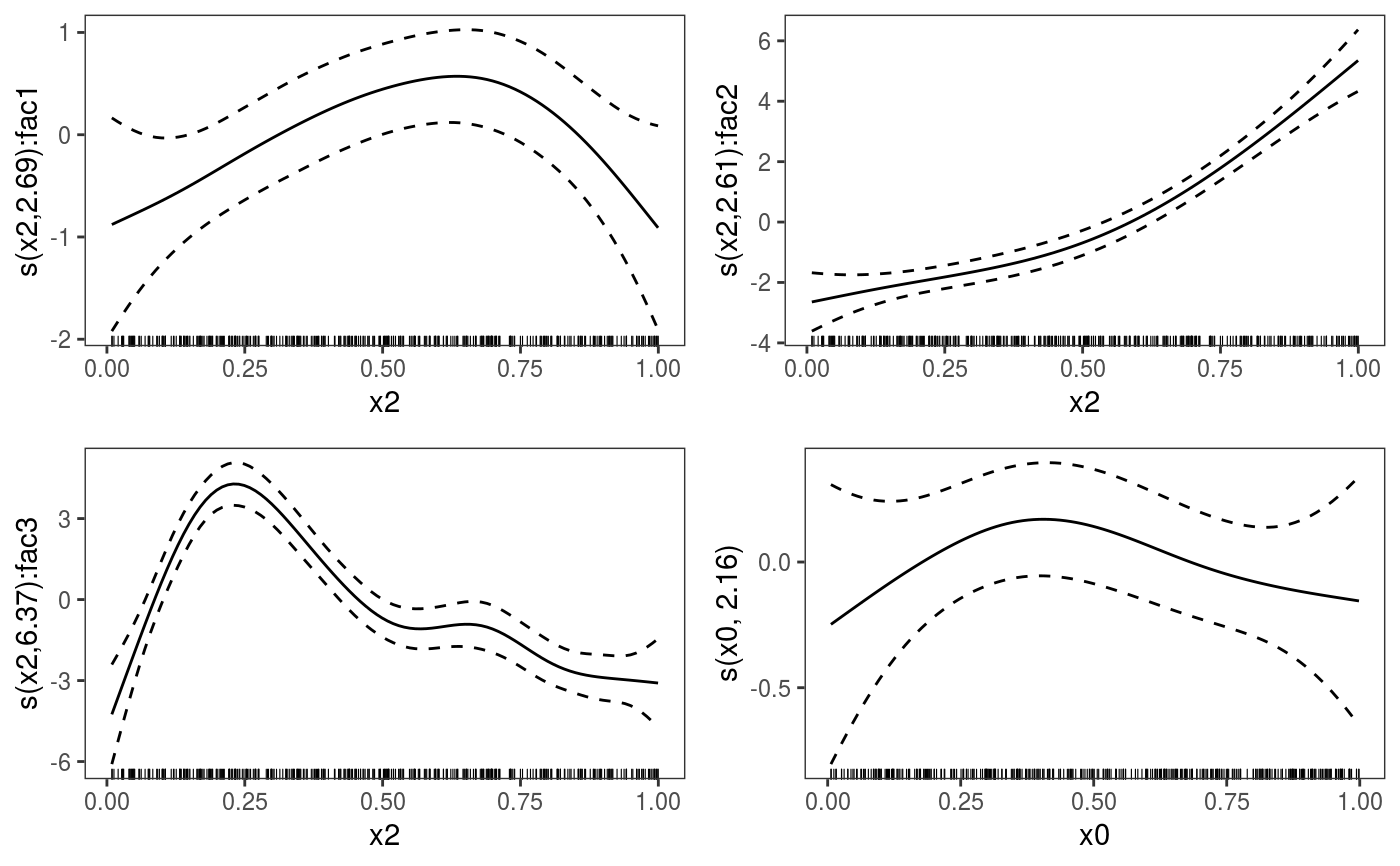
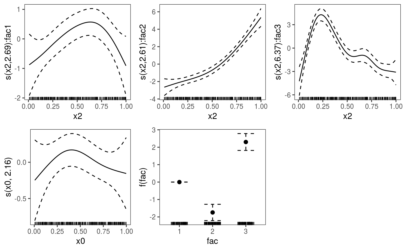
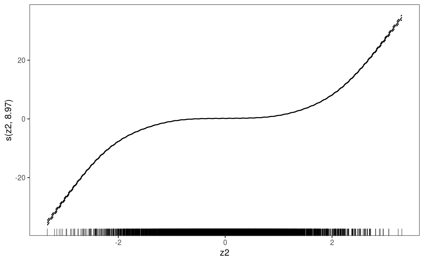
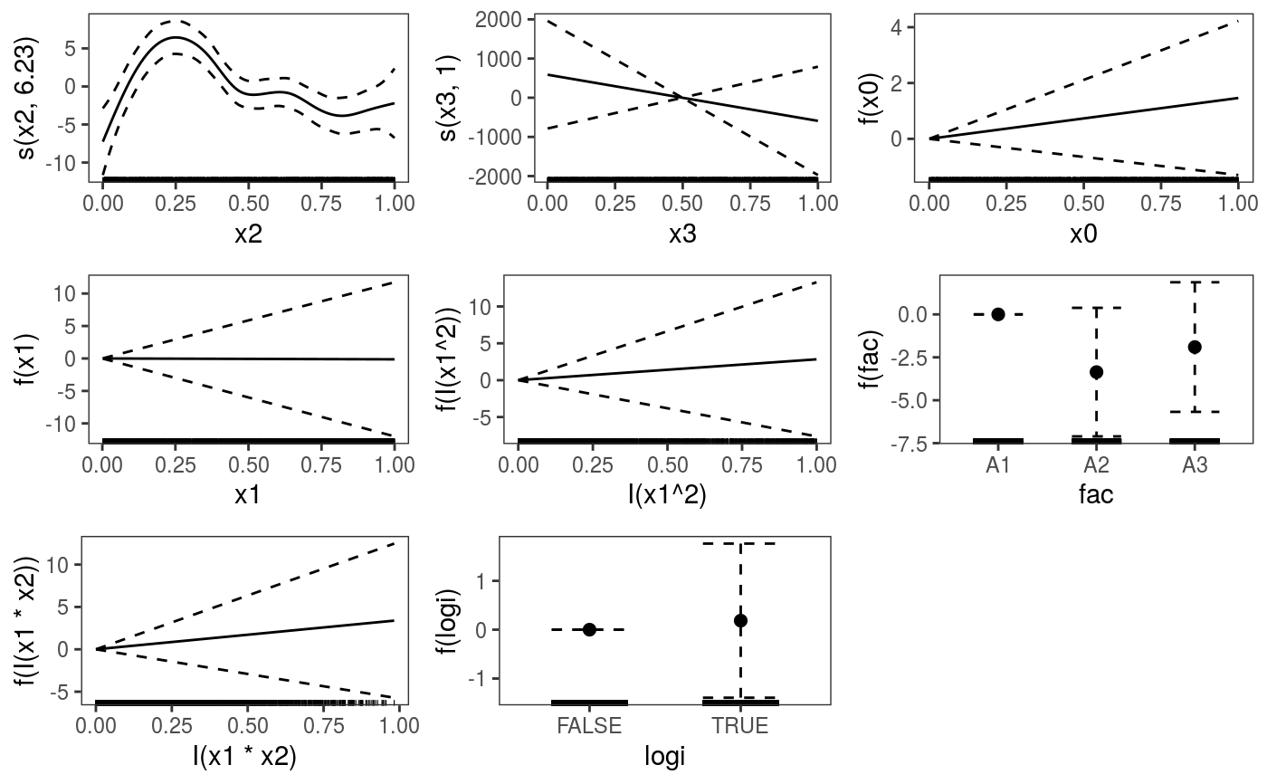
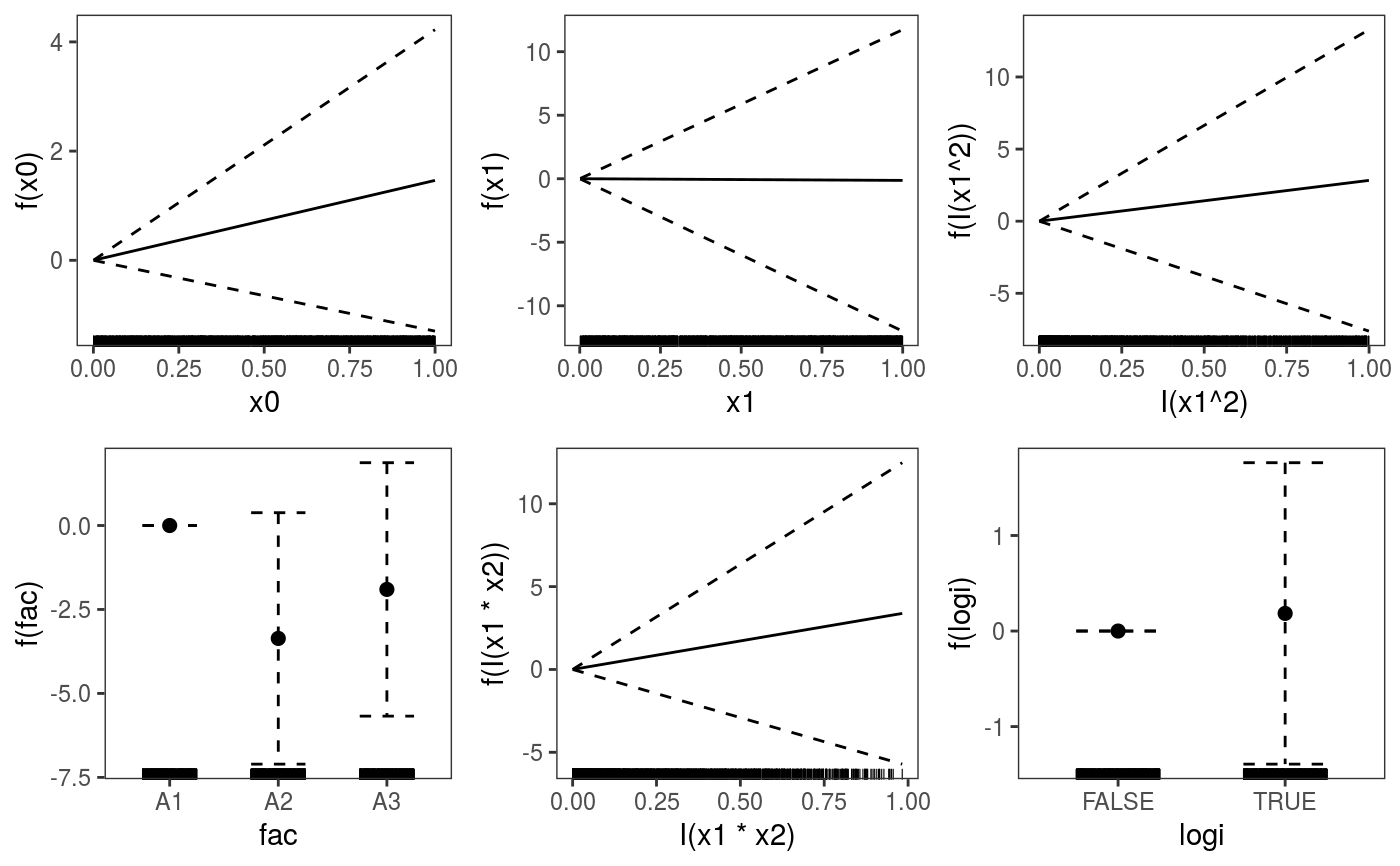
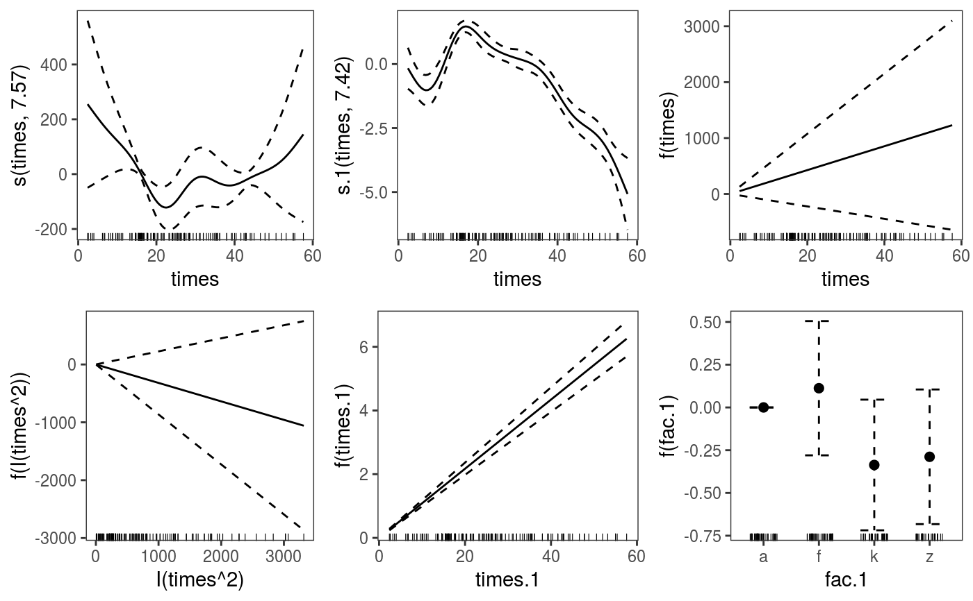
library(mgcViz)

######## Basic example
# Simulate some data and fit model
set.seed(2)
dat <- gamSim(1,n=1e3,dist="normal",scale=2)
#> Gu & Wahba 4 term additive model
b <- bam(y~s(x0)+s(x1, x2)+s(x3), data=dat)
b <- getViz(b)

# Default smooth effect plotting
print(plot(b), ask = FALSE)

# Now on one page and with out title on the second plot
print(plot(b) + labs(title = NULL), pages = 1)

# So far we used default layers, added in the printing phase, but
# we might want to specify our own layers. Here we is how to do it
pl <- plot(b) + l_points() + l_fitLine(linetype = 3) + l_fitContour() +
  l_ciLine(colour = 2) + theme_get() + labs(title = NULL)
print(pl, pages = 1)

# We might want to plot only the first smooth
plot(b, select = 1) + l_dens(type = "cond") + l_fitLine() + l_ciLine()

######## Example with "by variable" smooth effect
# Simulate data and fit model
dat <- gamSim(4)
#> Factor `by' variable example
b <- gam(y ~ fac+s(x2,by=fac)+s(x0),data=dat)
b <- getViz(b)
# print() only needed because we want to plot on a single page
print(plot(b), pages = 1)
print(plot(b, allTerms = TRUE), pages = 1) # Including also parametric effect

######## Example with 3D smooth effect which cannot be plotted
# Simulate data and fit model
n <- 5e3
x <- rnorm(n); y <- rnorm(n); z <- rnorm(n); z2 <- rnorm(n)

ob <- (x-z)^2 + (y-z)^2 + z2^3 + rnorm(n)
b1 <- bam(ob ~ s(x, y, z) + s(z2), discrete = TRUE)
b1 <- getViz(b1)

# Only second effect get plotted
plot(b1)
# In fact this does not plot anything
plot(b1, select = 1)
#> Nothing to plot!
# For plotting effects with more than 2D, one we need specific method. 
# See ?plot.mgcv.smooth.MD

######## Examples about plotting parametric effects
# 1 Gaussian GAM
set.seed(3)
dat <- gamSim(1,n=2500,dist="normal",scale=20)
#> Gu & Wahba 4 term additive model
dat$fac <- as.factor( sample(c("A1", "A2", "A3"), nrow(dat), replace = TRUE) )
dat$logi <- as.logical( sample(c(TRUE, FALSE), nrow(dat), replace = TRUE) )
bs <- "cr"; k <- 12
b <- bam(y ~ x0 + x1 + I(x1^2) + s(x2,bs=bs,k=k) + fac + x3:fac + I(x1*x2) + logi +
            s(x3, bs=bs),data=dat, discrete = TRUE)
b <- getViz(b)

# All effects in one page. Notably 'x3:fac' is missing: we have no methods
# for plotting second order effects.
print(plot(b, allTerms = TRUE), pages = 1)

# Plotting only parametric effects
print(plot(b, select = 3:9), pages = 1)

# 2 GAMLSS Gaussian model
library(mgcv);library(MASS)
mcycle$fac <- as.factor( sample(c("z", "k", "a", "f"), nrow(mcycle), replace = TRUE) )
b <- gam(list(accel~times + I(times^2) + s(times,k=10), ~ times + fac + s(times)),
          data=mcycle,family=gaulss())
b <- getViz(b)

# All effects on one page: effect of second linear predictor end with '.1'
print(plot(b, allTerms = TRUE), pages = 1)