Adding glyphs to 2D plots

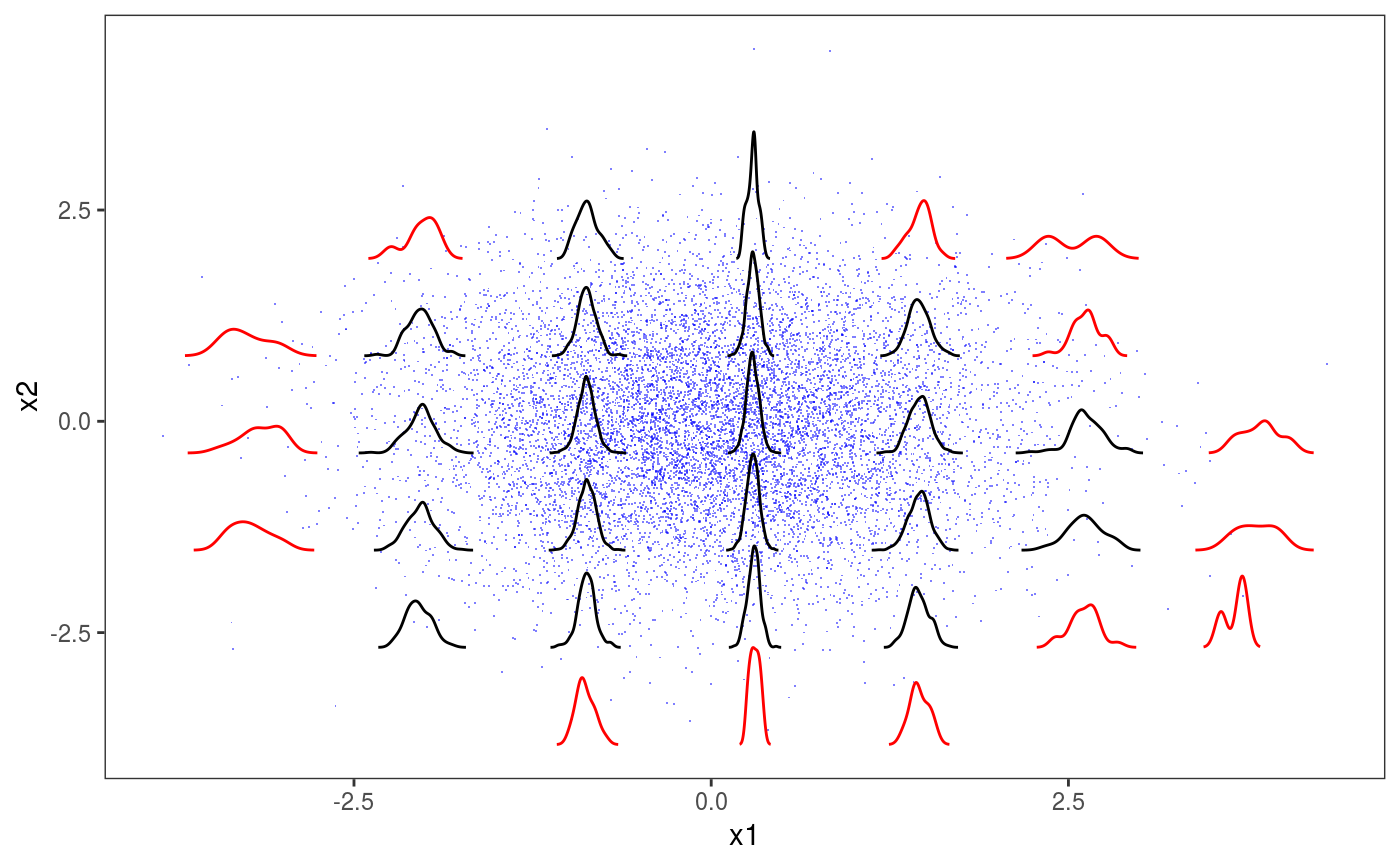
This layer adds glyphs or subplots to 2D plots. It is mainly meant to be used with check2D and to produce residuals checks.

l_glyphs2D(
  glyFun,
  ggLay = "geom_points",
  n = c(4, 4),
  mapping = NULL,
  data = NULL,
  polar = FALSE,
  height = ggplot2::rel(0.95),
  width = ggplot2::rel(0.95),
  y_scale = I,
  x_scale = I,
  ...
)

Arguments

glyFun	the function that produces the data needed to construct the glyphs. It will take a single argument (.d), which is a data.frame with columns "x", "y" and "z". When l_glyphs2D is used with check2D, then "x" and "y" will be the locations of the residual "z" in the relevant covariates. glyFun needs to output a data.frame that will be passed to the ggLay function, which does the plotting.
ggLay	the ggplot2 layer function (such as "geom_point") used to plot the glyphs. Its mapping needs to take at least argument "x", "y" and "group". See the mapping argument below.
n	vector of two positive integers, indicating the number of 2D grid cell along x and y in which the data is divided.
mapping	list of aesthetic mappings to be used by ggLay. By default it is aes(x=gx, y=gy, group = gid). Here gx and gy specify the x-y location of each data-point used to plot the glyphs, while gid specifies to which glyph each data-point belongs (there are n[1]*n[2] glyphs).
data	an optional data.frame to be used for computing the glyphs. It must have two variables called x and y. If left to NULL then the glyphs will be computed using the data in the plotSmooth object to which this layer is being added.
polar, height, width, y_scale, x_scale	see GGally::glyphs.
...	graphical arguments to be passed to ggLay function.

Value

An object of class gamLayer.

See also

check2D.

Examples

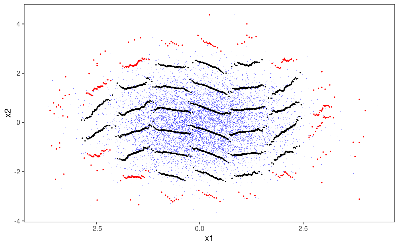
library(mgcViz);
set.seed(4124)
n <- 1e4
dat <- data.frame("x1" = rnorm(n), "x2" = rnorm(n))

# Residuals are heteroscedastic w.r.t. x1
dat$y <- (dat$x1)^2 + (dat$x2)^2 + (1*abs(dat$x1) + 1)  * rnorm(n)
b <- bam(y ~ s(x1,k=30) + s(x2, k=30), data = dat, discrete = TRUE)
b <- getViz(b)

pl <- check2D(b, x1 = "x1", x2 = "x2", type = "tnormal") +
  l_points(colour = "blue", alpha = 0.5)

# Look at distributions of residuals across x1 and x2
# Approach 1: using binned kernel density estimate
# Colour indicates whether we have more that 50 obs in that bin
glyFun <- function(.d){
  .r <- .d$z
  .qq <- as.data.frame( density(.r)[c("x", "y")], n = 100 )
  .qq$colour <- rep(ifelse(length(.r)>50, "black", "red"), nrow(.qq))
  return( .qq )
}

pl + l_glyphs2D(glyFun = glyFun, ggLay = "geom_path", n = c(8, 8),
                 mapping = aes(x=gx, y=gy, group = gid, colour = I(colour)),
                 height=1.5, width = 1)

# Approach 2: using binned worm-plots. These are simply rotated QQplots.
# An horizontal plot indicates well specified residual model. 
# Increasing (decreasing) worm indicates over (under) dispersion
glyFun <- function(.d){
  n <- nrow(.d)
  px <- qnorm( (1:n - 0.5)/(n) )
  py <- sort( .d$z )
  clr <- if(n > 50) { "black" } else { "red" }
  clr <- rep(clr, n)
  return( data.frame("x" = px, "y" = py - px, "colour" = clr))
}

pl + l_glyphs2D(glyFun = glyFun, ggLay = "geom_point", n = c(10, 10),
                mapping = aes(x=gx, y=gy, group = gid, colour = I(colour)),
                height=2, width = 1, size = 0.2)