Plotting slice of higher-dimensional smooth effects

This function plots a 2D slice of a higher-dimensional smooth effects.

# S3 method for mgcv.smooth.MD
plot(
  x,
  fix,
  n = 40,
  xlim = NULL,
  ylim = NULL,
  maxpo = 10000,
  too.far = c(0.1, NA),
  trans = identity,
  seWithMean = FALSE,
  unconditional = FALSE,
  ...
)

Arguments

x	a smooth effect object, extracted using mgcViz::sm.
fix	a named vector indicating which variables must be kept fixed and to what values. When plotting a smooth in (d+2) dimensions, then d variables must be fixed.
n	sqrt of the number of grid points used to compute the effect plot.
xlim	if supplied then this pair of numbers are used as the x limits for the plot.
ylim	if supplied then this pair of numbers are used as the y limits for the plot.
maxpo	maximum number of residuals points that will be used by layers such as resRug() and resPoints(). If number of datapoints > maxpo, then a subsample of maxpo points will be taken.
too.far	a numeric vector with two entries. The first has the same interpretation as in plot.mgcv.smooth.2D and it avoids plotting the smooth effect in areas that are too far form any observation. The distance will be calculated only using the variables which are not in fix (see above). Hence in two dimensions, not in the full d+2 dimensions. Set it to -1 to plot the whole smooth. The second entry determines which residuals and covariates pairs are closed enough to the selected slice. If left to NA on the 10\ closest (in terms of scaled Euclidean distance) to the current slice will be plotted. Set it to -1 to plot all the residuals.
trans	monotonic function to apply to the smooth and residuals, before plotting. Monotonicity is not checked.
seWithMean	if TRUE the component smooths are shown with confidence intervals that include the uncertainty about the overall mean. If FALSE then the uncertainty relates purely to the centred smooth itself. Marra and Wood (2012) suggests that TRUE results in better coverage performance, and this is also suggested by simulation.
unconditional	if TRUE then the smoothing parameter uncertainty corrected covariance matrix is used to compute uncertainty bands, if available. Otherwise the bands treat the smoothing parameters as fixed.
...	currently unused.

Value

An objects of class plotSmooth.

References

Marra, G and S.N. Wood (2012) Coverage Properties of Confidence Intervals for Generalized Additive Model Components. Scandinavian Journal of Statistics.

Examples

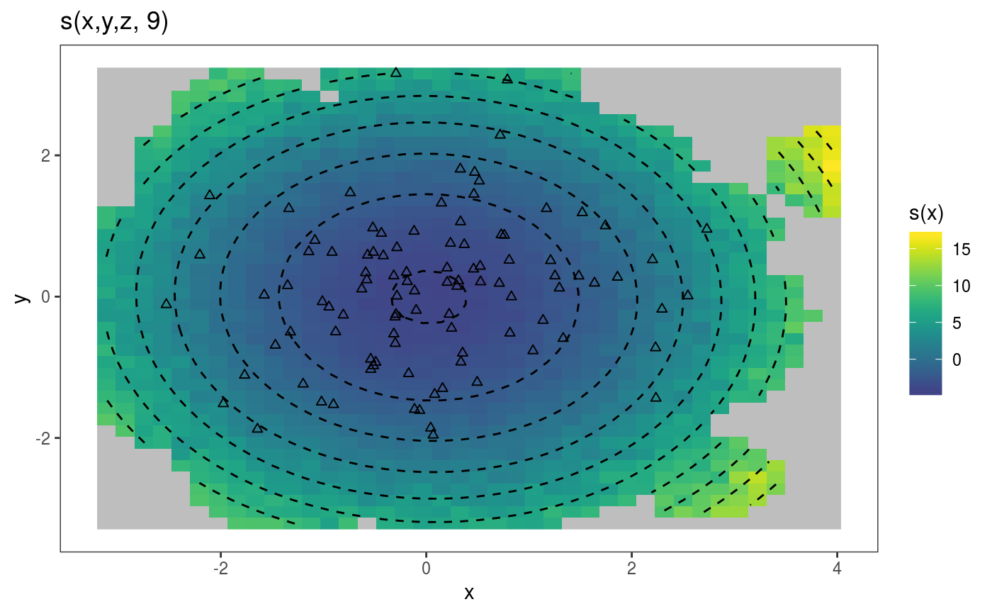
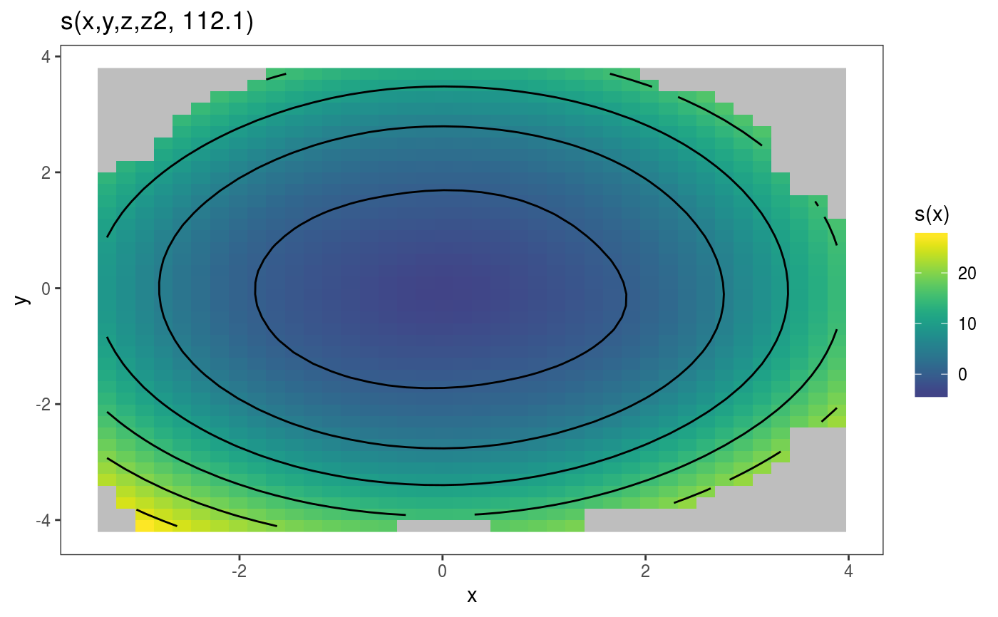
## 3D example
library(mgcViz)
n <- 1e3
x <- rnorm(n); y <- rnorm(n); z <- rnorm(n)

ob <- (x-z)^2 + (y-z)^2 + rnorm(n)
b <- gam(ob ~ s(x, y, z))
b <- getViz(b)

# Plot one 2D slice
plot( sm(b, 1), fix = c("z"=0) ) + l_fitRaster(noiseup = TRUE, mul = 3) +
  l_fitContour(linetype = 2) + l_points(shape =  2)

## 4D
n <- 5e3
x <- rnorm(n); y <- rnorm(n); z <- rnorm(n); z2 <- rnorm(n)

ob <- (x-z)^2 + (y-z)^2 + z2^3 + rnorm(n)
b1 <- bam(ob ~ s(x, y, z, z2), discrete = TRUE)
b1 <- getViz(b1)

# Plot one 2D slice
plot(sm(b1, 1), fix = c("z"=0, "z2"=1)) + l_fitRaster() + l_fitContour()