Posterior simulation from a GAM object

This method can be used to simulate vectors of responses from the Gaussian posterior approximation of a gamObject.

postSim(
  o,
  nsim,
  newdata,
  trans = NULL,
  method = "auto",
  w = NULL,
  offset = NULL,
  savePar = FALSE,
  ...
)

Arguments

o	the output of a gam() or bam() call.
nsim	the number of simulated vectors of responses. A positive integer.
newdata	Optional new data frame used to perform the simulations. To be passed to predict.gam.
trans	function used to transform or summarize each vector of simulated responses. It must take a vector as argument, but it can output a vector or a scalar. Potentially useful for saving storage (e.g. by transforming each simulated vector to a scalar). If left to NULL then trans = identity will be used.
method	the method used for the simulation of responses. See simulate.gam.
w	vector of prior weights of each response. See simulate.gam.
offset	numeric vector of offsets. For GAMs with multiple linear predictor (see eg gaulss) it must be a list of vectors. If newdata!=NULL the offsets will be assumed to be zero, unless their are explicitly provided. If newdata==NULL the simulations will use the offsets used during model fitting, unless offset is explicitly provided.
savePar	if TRUE than also the simulated parameters will be returned.
...	arguments to be passed to vcov.gam.

Value

If savePar == FALSE the function will return a matrix where each row is a vector of simulated responses or a transformed version of it. If savePar == TRUE it will return a list where the $simY entry will contain the simulated responses and $simBeta the simulated parameters.

Examples

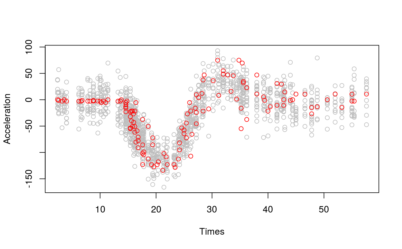
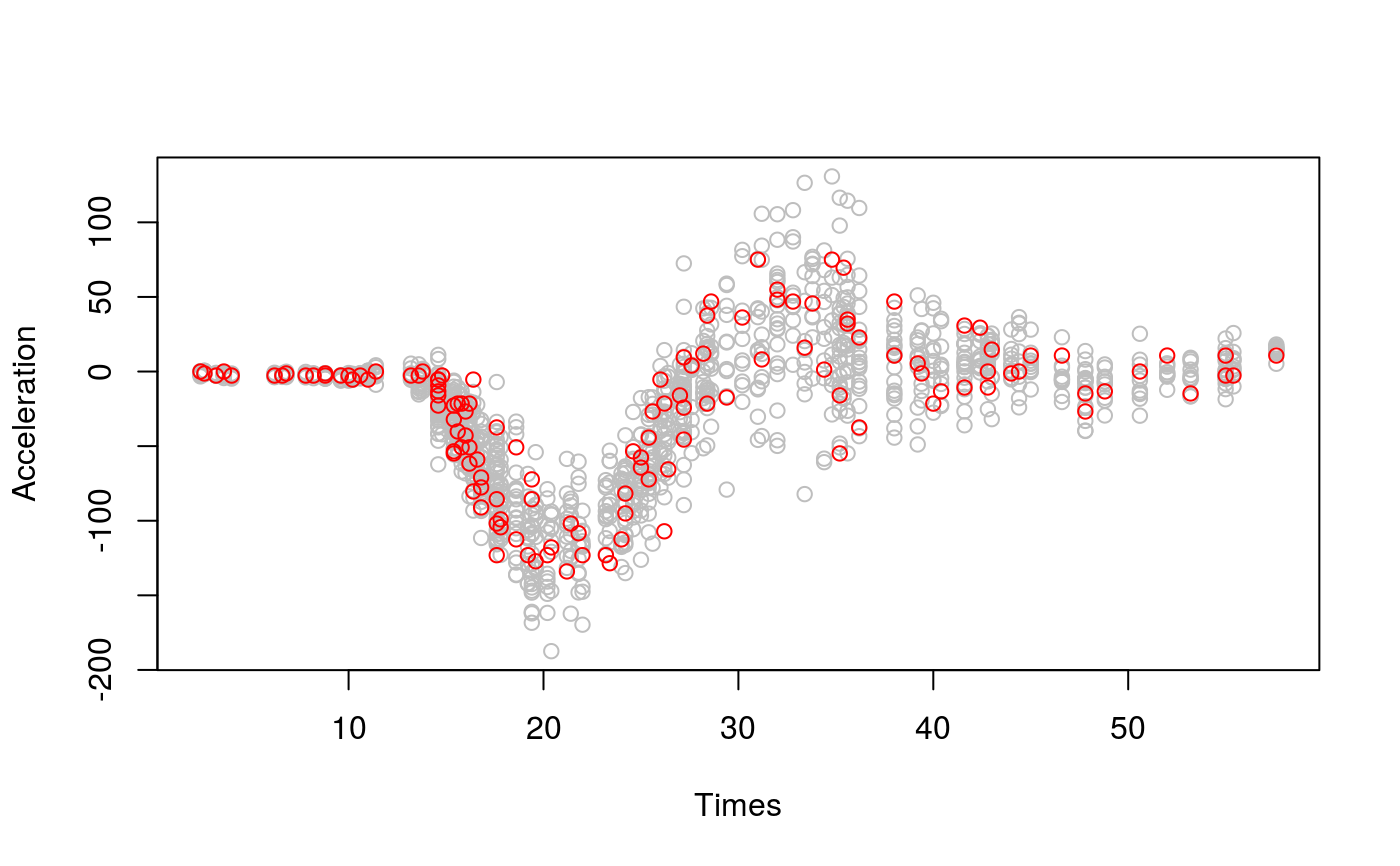
library(mgcViz)
library(MASS)
b <- gam(accel~s(times, k=20), data=mcycle)

# Simulate list of 10 vectors of responses from posterior, taking into
# account smoothing parameters uncertainty (see ?vcov.gam)
n <- 10
sim <- postSim(o = b, nsim = n, unconditional = TRUE)

# Posterior simulations in grey and data in red
plot(rep(mcycle$times, n), as.vector(t(sim)), col = "grey",
     ylab = "Acceleration", xlab = "Times")
points(mcycle$times, mcycle$accel, col = 2)

# There is clear disagreement between simulations' and data's 
# conditional variance, which can be solved using flexible GAMLSS model:
b <- gam(list(accel~s(times, k=20), ~s(times)), data=mcycle, family = gaulss)
sim <- postSim(o = b, nsim = n)
plot(rep(mcycle$times, n), as.vector(t(sim)), col = "grey",
     ylab = "Acceleration", xlab = "Times")
points(mcycle$times, mcycle$accel, col = 2)