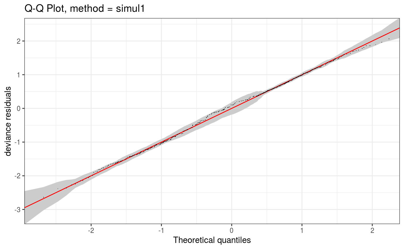
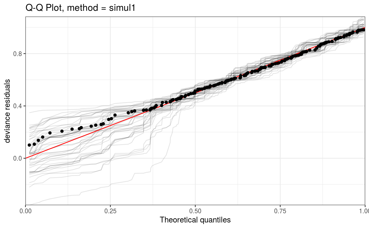
Efficiently zooming on GAM QQ-plots

This function allows to zoom into a QQ-plot produced by qq.gamViz, in a computationally efficient manner.

# S3 method for qqGam
zoom(
  o,
  xlim = NULL,
  ylim = NULL,
  discrete = NULL,
  ngr = 1000,
  adGrid = TRUE,
  CI = FALSE,
  worm = FALSE,
  showReps = FALSE,
  a.qqpoi = list(),
  a.ablin = list(),
  a.cipoly = list(),
  a.replin = list(),
  ...
)

Arguments

o	the output of `mgcViz::qq.gamViz`.
xlim	if supplied then this pair of numbers are used as the x limits for the plot.
ylim	if supplied then this pair of numbers are used as the y limits for the plot.
discrete	if `TRUE` the QQ-plot is discretized into `ngr` bins before plotting, in order to save plotting time (when the number of observations is large). If left to `NULL`, the discretization is used if there are more than 10^4 observations.
ngr	number of bins to be used in the discretization.
adGrid	if `TRUE` the discretization grid is computed using the QQ-points falling within `xlim`. If `FALSE`, `zoom.qqGam` will compute `ngr` values using all the QQ-points used in the original `qq.gamViz` call (but only those falling within `xlim` and `ylim` will be plotted).
CI	if `TRUE` confidence intervals are plotted.
worm	if `TRUE` a worm-plot (a de-trended QQ-plot) is plotted, rather than a QQ-plot.
showReps	if `TRUE` all the QQ-lines corresponding to the simulated (model-based) QQ-plots.
a.qqpoi	list of arguments to be passed to `ggplot2::geom_point`, which plots the main QQ-plot.
a.ablin	list of arguments to be passed to `ggplot2::geom_abline`, which adds the reference line.
a.cipoly	list of arguments to be passed to `ggplot2::geom_polygon`, which add the confidence intervals.
a.replin	list of arguments to be passed to `ggplot2::geom_line`, which adds a line for each simulated QQ-plot.
...	currently unused.

Examples

library(mgcViz);
set.seed(0)
n.samp <- 500
dat <- gamSim(1,n=n.samp,dist="binary",scale=.33)
#> Gu & Wahba 4 term additive model
p <- binomial()$linkinv(dat$f) ## binomial p
n <- sample(c(1,3),n.samp,replace=TRUE) ## binomial n
dat$y <- rbinom(n,n,p)
dat$n <- n
lr.fit <- bam(y/n ~ s(x0) + s(x1) + s(x2) + s(x3)
              , family = binomial, data = dat,
              weights = n, method = "REML")
lr.fit <- getViz(lr.fit)

set.seed(414)
o <- qq(lr.fit, rep = 50, method = "simul1", CI = "normal")
o # This is the whole qqplot

# We can zoom in along x at little extra costs (most computation already done by qq.gamViz)
zoom(o, xlim = c(0, 1), showReps = TRUE,
     a.replin = list(alpha = 0.1), a.qqpoi =  list(shape = 19))

Arguments

Examples

Contents