Binning and checking QGAM residuals

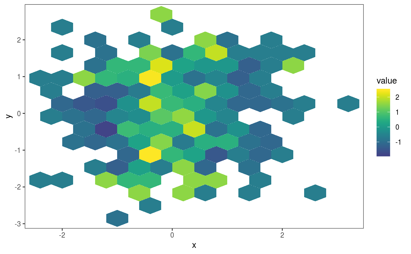
This layer bins the residuals, r, according to the value of the corresponding covariates, x1 and x2. Then we calculate the proportion of negative residuals in each bin, which should not deviate too much from the theoretical proportion (eg 0.5 if we fit the median). Mainly useful in conjuction with check2D.

l_gridQCheck2D(qu = NULL, bw = c(NA, NA), stand = TRUE, binFun = NULL, ...)

Arguments

qu	the quantile of interest. Should be in (0, 1).
bw	numeric vector giving bin width in the vertical and horizontal directions. See the binwidth arguments in ?ggplot2::stat_summary_hex. If left to NA, it will be set to 1/20 of the ranges of x1 and x2.
stand	if left to TRUE then the observed proportion of negative residuals p_hat in the i-th cell is normalized using the standard error se = sqrt(qu(1-qu)/n), where n is the number of observation in that cell. That is, if stand=TRUE we plot (p_hat-qu)/se rather than simply p_hat.
binFun	the ggplot2 function used to perform the binning. By default it is either ggplot2::stat_summary_2d or ggplot2::stat_summary_hex, depending on the class of the covariates x1 and x2.
...	graphical arguments to be passed to ggplot2::stat_summary_hex.

Value

An object of class gamLayer

Examples

library(mgcViz);
set.seed(4124)
n <- 4e2
dat <- data.frame(x = rnorm(n), y = rnorm(n))

# Simulate some data, residuals are heteroscedastic w.r.t. x
dat$ob <- (dat$x)^2 + (dat$y)^2 + (0.2*abs(dat$x) + 1)  * rnorm(n)
b <- qgamV(ob ~ x + s(y), qu = 0.3, data = dat)
#> Estimating learning rate. Each dot corresponds to a loss evaluation. 
#> qu = 0.3........done 

# We have a residual pattern along x (increase n above to 
# see the problem more clearly) 
check2D(b, "x", "y") + l_gridQCheck2D(qu = 0.3, bw = c(0.4, 0.4))

# We need a smooth wrt x to make the pattern disappear
if (FALSE) {
b1 <- qgamV(ob ~ s(x) + s(y), qu = 0.3, data = dat)

check2D(b1, "x", "y") + l_gridQCheck2D(qu = 0.3, bw = c(0.4, 0.4))
}