Plotting multiple quantile GAMs

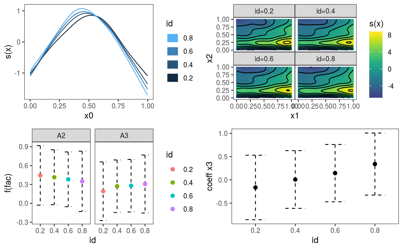
This function is similar to plot.gamViz, but it is used to plot multiple quantile GAM models fitted using mqgamV or mqgam. It allows plotting standards 1D and 2D smooths, and parametric effects, It is basically a wrapper around plotting methods that are specific to individual smooth effect classes (such as plot.multi.mgcv.smooth.1D).

# S3 method for mgamViz
plot(x, n = 100, n2 = 40, select = NULL, allTerms = FALSE, ...)

Arguments

x	an object of class `mgamViz`, the output of a getViz call. Alternatively x can be a list of fitted GAM models, each having the same model formula.
n	number of points used for each 1-d plot. For a nice smooth plot this needs to be several times the estimated degrees of freedom for the smooth.
n2	square root of number of grid points used for plotting 2D functions effects using contours or heatmaps.
select	allows plotting a subset of model terms. For instance, if you just want the plot for the second smooth term, set `select = 2`. Parametric effects always come after smooth or random effects.
allTerms	if `TRUE` also the parametric effects will be plotted.
...	other parameters, such as `maxpo` or `trans`, to be passed to the specific plotting methods for each effect (e.g. to plot.multi.mgcv.smooth.1D).

Value

An object of class c("plotGam", "gg").

Examples

library(mgcViz)
set.seed(2) ## simulate some data...
dat <- gamSim(1,n=500,dist="normal",scale=2)
#> Gu & Wahba 4 term additive model
dat$logi <- as.logical( sample(c(TRUE, FALSE), nrow(dat), replace = TRUE) )

dat$fac <- as.factor( sample(c("A1", "A2", "A3"), nrow(dat), replace = TRUE) )

# Fit GAM and get gamViz object
fit <- mqgamV(y ~ fac + s(x0) + s(x1, x2) + x3 + logi, data = dat,
              qu = c(0.2, 0.4, 0.6, 0.8))
#> Estimating learning rate. Each dot corresponds to a loss evaluation. 
#> qu = 0.4........done 
#> qu = 0.6.........done 
#> qu = 0.2.........done 
#> qu = 0.8..........done 

print(plot(fit, select = 1:4, allTerms = T), pages = 1)

if (FALSE) {
# Example where we are fitting the same model to different datasets, but
# plotting the estimate effects together 
dat <- list()
for(ii in 1:4){
  # Simulate 4 datasets, we are adding 2 factor variables "fac" and "ref" just
  # for illustrating the plotting method (the two factors have no effect on y)
  n <- 1000
  dat[[ii]] <- gamSim(1,n=n,dist="normal",scale=2)
  dat[[ii]]$fac <- as.factor( sample(c("A1", "A2", "A3"), n, replace = TRUE) )
  dat[[ii]]$ref <- as.factor( sample(letters[1:10], n, replace = TRUE) )
}

# Estimating model on each dataset
mods <- list()
for(ii in 1:4){
  mods[[ii]] <- gamV(y~s(x0)+s(x1, x2)+x3+fac+s(ref, bs = "re"), data = dat[[ii]])
}

# Names will be used to identify the four models we have fitted 
names(mods) <- c("M1", "M2", "M3", "M4")
# Plotting on the same plots
print(plot.mgamViz(mods, allTerms = TRUE), pages = 1)
}

Arguments

Value

Examples

Contents